Linear Regression Explained with Real Life Example

In this post, the linear regression concept in machine learning is explained with multiple real-life examples. Both types of regression models (simple/univariate and multiple/multivariate linear regression) are taken up for sighting examples. In case you are a machine learning or data science beginner, you may find this post helpful enough. You may also want to check a detailed post on what is machine learning – What is Machine Learning? Concepts & Examples.

Before going into the details, lets look at a small poem which can help us remember the concept of linear regression. Hope you like it.

Linear Regression, a machine learning delight
Fitting a line, to make predictions right
Training on data, with features and label
Minimizing error, for a model stable

With a slope and intercept, it’s easy to see
How well it predicts, with accuracy degree
Ordinary Least Squares, a method so neat
Solving for coefficients, that can’t be beat

Outliers can be trouble, for this method divine
Robust regression, can help to align
But with assumptions in check, and data clean
Linear Regression, a powerful machine

What is Linear Regression?

Linear regression is a machine learning concept that is used to build or train the models (mathematical models or equations)  for solving supervised learning problems related to predicting continuous numerical value. Supervised learning problems represent the class of the problems where the value (data) of the independent or predictor variable (features) and the dependent or response variables are already known. The known values of the dependent and independent variable (s) are used to come up with a mathematical model/formula also called as linear regression equation which is later used to predict / estimate output given the value of input features (independent variable). In machine learning tasks, linear regression is used for making the prediction of numerical values from a set of input values. The following is an example of linear univariate linear regression analysis representing the relationship between the height and weight in adults using the regression line. The regression line is superimposed over the scatterplot of height vs weight to showcase the linear relationship.

Building linear regression models represents determining the value of output (dependent/response variable) as a function of the weighted sum of input features (independent / predictor variables).  This data is used to determine the most optimum value of the coefficients of the independent variables.

Here are few assumptions which need to be kept in mind when building linear regression models:

• The linear regression mathematical structure or model assumes that there is a linear relationship between input and output variables.
• It is also assumed that the noise or residual error is well-mannered (normal or Gaussian distribution).

Let’s say, there is a numerical response variable, Y, and one or more predictor variables X1, X2, etc. And, there is some relationship between Y and X that can be written as the following:

[latex]Y_i = f(X) + error[/latex]

Where [latex]Y_i[/latex] is the actual or observed value and  f is some fixed but unknown function of X1 and X2 which is used to come up with predicted value [latex]\hat{Y_i}[/latex]. The difference between the actual or observed value, [latex]Y_i[/latex] and the predicted value, [latex]\hat{Y_i}[/latex] is called as the error or residual. When the unknown function is a linear function of X1 and X2, the Y becomes a linear regression function or model such as the following. Note that the error term averages out to be zero.

[latex]\hat{Y_i} = b0 + b1*X1 + b2*X2[/latex] 

In the above equation, different values of Y and X1, and X2 are known during the model training phase. As part of training the model, the most optimal value of coefficients b1, b2, and b0 are determined based on the least square regression algorithm. The least-squares method is an algorithm to find the best fit for a set of data points by minimizing the sum of the squared residuals or square of error of points (actual values representing the response variable) from the points on the plotted curve (predicted value). This is shown below.

If [latex]Y_i[/latex] is the ith observed value and [latex]\hat{Y_i}[/latex] is the ith predicted value, then the ith residual or error value is calculated as the following:

[latex]e_i = Y_i – \hat{Y_i} [/latex]

The residual sum of squares can then be calculated as the following:

[latex]RSS = {e_1}^2 + {e_2}^2 + {e_3}^2 + … + {e_n}^2[/latex]

In order to come up with the optimal linear regression model, the least-squares method as discussed above represents minimizing the value of RSS (Residual sum of squares).

In order to select the most appropriate variables / features such as X1, X2, etc., the hypothesis is laid down around the coefficient for each of the variables / features. The null hypothesis is that the value of coefficients are 0. This means that the value of b0, b1, b2, etc. are 0. The alternate hypothesis is that the coefficients are not equal to zero. In this manner, the dependent variable holds good. T-statistics is used for hypothesis testing and reject the null hypothesis (b0, b1 or b2 = 0) if appropriate. The following is the formula of the t-statistics with n-2 degree of freedom. For more details, read my related blog –  linear regression and t-test.

[latex]t = \frac{b_i}{StandardError(b_i)}[/latex]

Different types of linear regression models

There are two different types of linear regression models. They are the following:

• Simple linear regression: The following represents the simple linear regression where there is just one independent variable, X, which is used to predict the dependent variable Y.
  

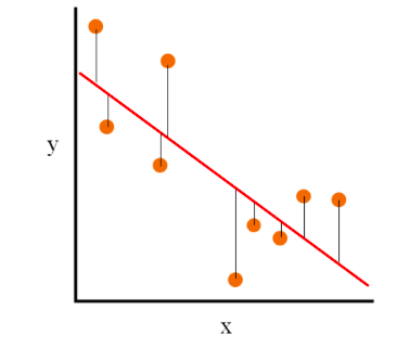
  Fig 1. Simple linear regression

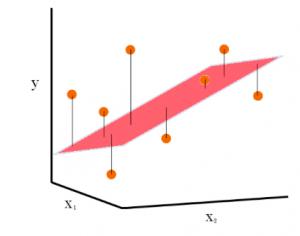
• Multiple linear regression: The following represents the multiple linear regression where there are two or more independent variables (X1, X2) that are used for predicting the dependent variable Y.
  

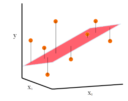
  Fig 2. Multiple linear regression

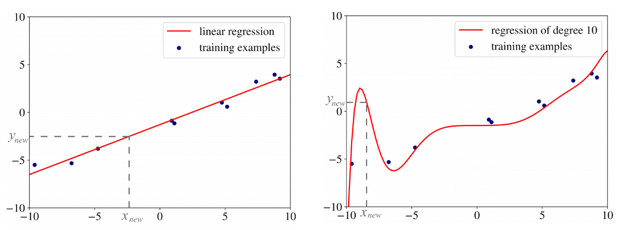
We have seen that the linear regression model is learned as the linear combination of features to predict the value of the target or response variable. However, we could use a square or some other polynomial to combine the values of features and predict the value of the target variable. This would turn out to be a more complex model than the linear one. One of the reasons why the linear regression model is more useful than the polynomial regression is the fact that the polynomial regression overfits. The picture below represents the linear vs polynomial regression model and represents how the polynomial regression model tends to overfit.

Simple Linear Regression Example

As shown above, simple linear regression models comprise of one input feature (independent variable) which is used to predict the value of the output (dependent) variable. The following mathematical formula represents the regression model:

[latex]Y_i = b*{X_i} + b_0 + error[/latex]

where [latex]Y_i[/latex] represents the observed value. Let’s take an example comprising one input variable used to predict the output variable. However, in real life, it may get difficult to find a supervised learning problem that could be modeled using simple linear regression.

Simple Linear Model for Predicting Marks

Let’s consider the problem of predicting the marks of a student based on the number of hours he/she put into the preparation. Although at the outset, it may look like a problem that can be modeled using simple linear regression, it could turn out to be a multiple linear regression problem depending on multiple input features. Alternatively, it may also turn out to be a non-linear problem. However, for the sake of example, let’s consider this as a simple linear regression problem.

However, let’s assume for the sake of understanding that the marks of a student (M) do depend on the number of hours (H) he/she put up for preparation. The following formula can represent the model:

Marks = function (No. of hours)

=> Marks = m*Hours + c

The best way to determine whether it is a simple linear regression problem is to do a plot of Marks vs Hours. If the plot comes like below, it may be inferred that a linear model can be used for this problem.

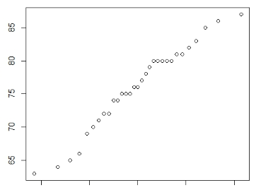
Fig 3. Plot representing a simple linear model for predicting marks

The data represented in the above plot would be used to find out a line such as the following which represents a best-fit line. The slope of the best-fit line would be the value of “m”.

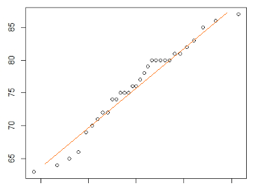
Fig 4. Plot representing a simple linear model with a regression line

The value of m (slope of the line) can be determined using an objective function which is a combination of the loss function and a regularization term. For simple linear regression, the objective function would be the summation of Mean Squared Error (MSE). MSE is the sum of squared distances between the target variable (actual marks) and the predicted values (marks calculated using the above equation). The best fit line would be obtained by minimizing the objective function (summation of mean squared error).

Multiple Linear Regression Example

Multiple linear regression can be used to model the supervised learning problems where there are two or more input (independent) features that are used to predict the output variable. The following formula can be used to represent a typical multiple regression model:

[latex]Y_i = b_0 + b_1*X_1 + b_2*X_2 + b_3*X_3 + … + b_n*X_n + error[/latex] 

In the above example, [latex]Y_i[/latex] represents the observed value, and X1, X2, and X3 represent the input features. The model (mathematical formula) is trained using training data to find the optimum values of b0, b1, b2, and b3 which minimizes the objective function (mean squared error).

Multiple Linear Regression Model for Predicting Weight Reduction

The problem of predicting weight reduction in form of the number of KGs reduced, hypothetically, could depend upon input features such as age, height, the weight of the person, and the time spent on exercises, .

Weight Reduction = Function(Age, Height, Weight, TimeOnExercise)

=> Shoe-size = b1*Height + b2*Weight + b3*age + b4*timeOnExercise + b0

As part of training the above model, the goal would be to find the value of b1, b2, b3, b4, and b0 which would minimize the objective function. The objective function would be the summation of mean squared error which is nothing but the sum of the square of the actual value and the predicted value for different values of age, height, weight, and timeOnExercise.

Key Terminologies for Regression Models

The following are some key terminologies in relation to measuring the residuals and performance of the linear regression models:

• Root Mean Square Error (RMSE): Root Mean Square Error (RMSE) is a measure of how well a linear regression model fits the data. It is calculated by taking the squared difference between the predicted values and the observed values, finding an average of all the differences, and then taking the square root of this number. The lower the RMSE value, the better fit of our model to the data.
  
• R-Squared: R-Squared is a statistical measure that represents how well the linear regression model fits the data. It is also known as the coefficient of determination. It is a statistic that measures the proportion of variation in the dependent variable (the y-axis) that can be explained by the independent variables (the x-axis). The R-squared value ranges between 0 and 1, with 1 indicating a perfect fit. A higher R-squared value indicates that more of the variance in the dependent variable can be explained by the independent variables.
  
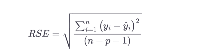
• Residual standard error (RSE): Residual Standard Error (RSE) is a measure of how well linear regression models fit the data. It is calculated by taking the sum of the squared residuals (the differences between the observed values and predicted values), dividing it by the degrees of freedom, then taking its square root. The RSE provides an indication of how much variation there is in the data that cannot be explained by the regression model. Lower RSE values indicate better fits to the data.
  

Assumptions for Linear Regression Models

While working with linear regression models, some of the following assumptions are made about the data. If these assumptions are violated, the results of linear regression analysis might not turn out to be valid:

• Linearity: The relationship between the predictor and the response variable would resemble a straight line. This assumption is checked by scatter plotting the data. If the plot resembles a shape other than the straight line, it might require transforming one or more variables.
• Data appropriateness: The values of response variable must be continuous and unbounded (cover a wide range of values). The values of independent variables must as well be continuous and dichotomous. Categorical variables having more than two values must be converted into a series of dichotomous dummy variables.
• Data independence: Each of the value of response variable would be independent of each other’s value. This assumption can be checked against scenario such as time-dependency or values of response variables forming clusters, etc.
• Data distribution: It is assumed that the response variable is normally distributed. In other words, the response variable follows Gaussian distribution. The distribution can be checked by creating a histogram (eyeballing the data) and by a statistical test for normality such as the Kolmogorov-Smirnov.
• Homoscedasticity: The prediction errors remain nearly constant & consistent regardless of how far the data range extends. It essentially means that the prediction errors don’t change with the value of response variable. For instance, for smaller values of response variable (Y), the prediction error will be small and for larger values, it becomes large. This can be ascertained by plotting standardized residuals against their corresponding predicted values – any significant changes in error size would be immediately visible.

Real-world examples of linear regression models

The following represents some real-world examples / use cases where linear regression models can be used:

• Forecasting sales: Organizations often use linear regression models to forecast future sales. This can be helpful for things like budgeting and planning. Algorithms such as Amazon’s item-to-item collaborative filtering are used to predict what customers will buy in the future based on their past purchase history.
• Cash forecasting: Many businesses use linear regression to forecast how much cash they’ll have on hand in the future. This is important for things like managing expenses and ensuring that there is enough cash on hand to cover unexpected costs.
• Analyzing survey data: Linear regression can also be used to analyze survey data. This can help businesses understand things like customer satisfaction and product preferences. For example, a company might use linear regression to figure out how likely people are to recommend their product to others.
• Stock predictions: A lot of businesses use linear regression models to predict how stocks will perform in the future. This is done by analyzing past data on stock prices and trends to identify patterns.
• Predicting consumer behavior: Businesses can use linear regression to predict things like how much a customer is likely to spend. Regression models can also be used to predict consumer behavior. This can be helpful for things like targeted marketing and product development. For example, Walmart uses linear regression to predict what products will be popular in different regions of the country.
• Analysis of relationship between variables: Linear regression can also be used to identify relationships between different variables. For example, you could use linear regression to find out how temperature affects ice cream sales.

References – Further Reads

Here are some of my other posts in relation to linear regression:

• Building linear regression models
  • Linear regression explained with python examples: The concepts such as residual error, SSE (Sum of squares residual error), SSR (Sum of Squares Regression), SST (Sum of Squares Total), R-Squared, etc have been discussed with diagrams. A linear regression model is trained with Sklearn Boston housing data set using Sklearn.linear_model LinearRegression implementation
• Assessing regression model performance
  • R-squared in linear regression – Concepts, Examples: This blog describes the concepts of R-squared which is a metric used for assessing the performance of linear regression model. R-squared represents the fraction of variance explained by the regression model.
  • R-squared vs Adjusted R-squared – Differences, Examples: This blog describes the concepts of R-squared and adjusted R-squared along with the differences and why you should choose one over the other.
  • Mean Squared Error (MSE) or R-Squared: Which one to use?: Linear regression model performance metrics such as MSE and R-Squared with Python code examples have been discussed.
• Linear regression & hypothesis testing
  • Linear regression hypothesis testing example: This blog post explains concepts in relation to how T-tests and F-tests are used to test different hypotheses in relation to the linear regression model. T-tests are used to test whether there is a relationship between response and individual predictor variables. F-test is used to test whether there exists a linear regression model representing the problem statement.
  • Linear regression & T-test: The blog post explains the concepts in relation to how T-tests are used to test the hypotheses related to the relationship between response and predictor variables.
  • How to interpret F-statistics in linear regression model: This blog explains the concepts of F-statistics and how they can be used to test the hypothesis whether there exists a linear regression comprising of predictor variables.

Summary

In this post, you learned about linear regression, different types of linear regression, and examples for each one of them. It can be noted that a supervised learning problem where the output variable is linearly dependent on input features could be solved using linear regression models. Linear regression models get trained using a simple linear or multiple linear regression algorithm which represents the output variable as the summation of weighted input features.