There are two measures of the strength of linear regression models: adjusted r-squared and r-squared. While they are both important, they measure different aspects of model fit. In this blog post, we will discuss the differences between adjusted r-squared and r-squared, as well as provide some examples to help illustrate their meanings. As a data scientist, it is of utmost importance to understand the differences between adjusted r-squared and r-squared in order to select the most appropriate linear regression model out of different regression models.
What is R-squared?
R-squared, also known as the coefficient of determination, is a measure of what proportion of the variance in the value of the dependent or response variable is explained by one or more independent or predictor variables in the regression model. In other words, R-squared is a measure of how close the data are to the fitted regression line. It takes a value between 0 and 1 (or 0% and 100%), where:
- An R-squared of 1 or 100% indicates that all changes in the dependent variable are completely explained by changes in the independent variable(s). However, it’s important to note that a high R-squared does not necessarily indicate that the model has a good fit. That might be the case if the model is overfitted, for instance.
- An R-squared of 0 or 0% indicates that the independent variable(s) explain none of the variability of the dependent / response variable.
Mathematically, the value of R-squared can be calculated as ratio of explained variance (SSR) to the total variance. and the following:
R-squared = sum of squares regression (SSR) / sum of squares total (SST)
Where:
- The total sum of squares (SST) is the total variance in the dependent variable (Y) from its mean. It’s the sum of the squared differences between the actual Y and the mean of Y.
- The sum of squares regression (SSR) is the total variance in the dependent variable (Y) that can be explained by the independent variable(s) (X). It’s the sum of the squared differences between the predicted Y and the mean of Y.
It can also be calculated using the following formula as a function of residuals.
R-squared =1 – (sum of squares residuals error (SSE) / sum of squares total (SST))
Where:
- Sum of squares residual error (SSE) is the total variance in the dependent variable (Y) that cannot be explained by the independent variable(s) (X). It’s the sum of the squared differences between the actual Y and the predicted Y.
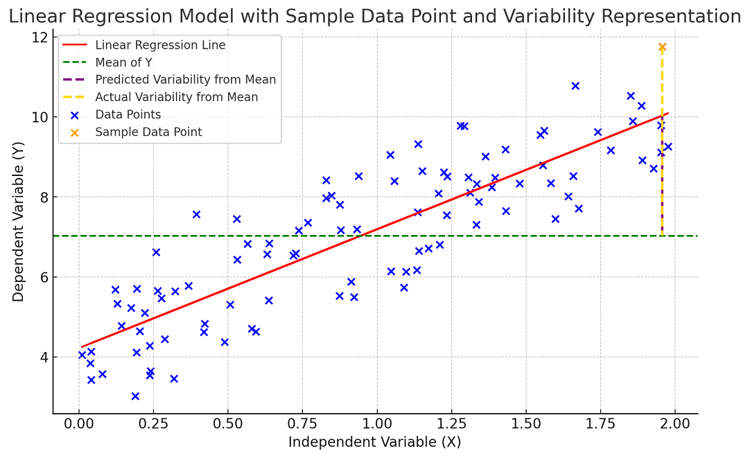
The following picture would help you understand the concept of R-squared in a better manner. Note that orange dashed line represent SST and brown dashed line represent SSR.
The value of R-squared increases with the increase in the number of independent variables used in the regression model. However, it does not mean that more is always better because adding an additional variable to the regression model might increase R-squared but at the same time not necessarily improve the model performance model. This is where the concept of adjusted r-squared comes into the picture. In the next section, we will learn about the adjusted R-squared.
Calculating R-Squared Value: Python Example
Here is how we can use Python and the sklearn library to perform a linear regression on the Boston Housing Dataset and calculate R-squared:
import pandas as pd
from sklearn.model_selection import train_test_split
from sklearn.linear_model import LinearRegression
from sklearn.metrics import r2_score
# Load the Boston housing dataset
url = "https://raw.githubusercontent.com/selva86/datasets/master/BostonHousing.csv"
data = pd.read_csv(url)
# Split the data into predictors and target
X = data.drop('medv', axis=1)
y = data['medv']
# Split the data into training set and test set
X_train, X_test, y_train, y_test = train_test_split(X, y, test_size=0.2, random_state=42)
# Create a Linear Regression model and fit it to the training data
model = LinearRegression()
model.fit(X_train, y_train)
# Use the model to make predictions on the test set
y_pred = model.predict(X_test)
# Calculate the R-squared score
r2 = r2_score(y_test, y_pred)
print(f'R-squared: {r2}')
What is Adjusted R-squared?
Adjusted r-squared can be defined as the proportion of variance explained by the model while taking into account both the number of predictor variables and the number of samples used in the regression analysis. The adjusted r-squared increases only when adding an additional variable to the model improves its predictive capability more than expected by chance alone. Adjusted R-squared is always less than or equal to R-squared.
The idea behind adjusted R-squared is to account for the addition of variables that do not significantly improve the model. When more and more predictor variables are added to the model, the R-squared will generally increase (even if those variables are only weakly associated with the response). This can give a misleading impression of improving model fit. Adjusted R-squared controls for this by penalizing the addition of uninformative predictors.
Mathematically, adjusted r-squared can be calculated as the function of R-squared in the following manner:
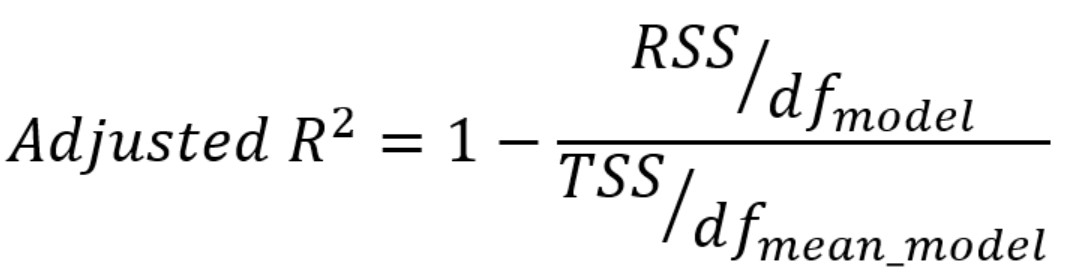
RSS represents the residual sum of squares or sum of squares residual error
TSS represents the total sum of squares or sum of squares total
DFmodel = Degrees of freedom for the regression model = N – P – 1, where P is the number of predictor variables and N is the number of records
DFmean_model = Degrees of freedom for the model representing the mean of the values of response variables = N – 1, where N is the number of records.
The above formula will thus become the following:
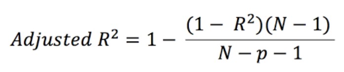
Note that (1 – R-squared) is the same as RSS/TSS or SSE / SST.
Python Code for Calculating Adjusted R-Squared
The following code demonstrates how we can calculate both R-squared and adjusted R-squared in Python using the sklearn library and the Boston Housing Dataset:
import pandas as pd
from sklearn.model_selection import train_test_split
from sklearn.linear_model import LinearRegression
from sklearn.metrics import r2_score
# Load the Boston housing dataset
url = "https://raw.githubusercontent.com/selva86/datasets/master/BostonHousing.csv"
data = pd.read_csv(url)
# Split the data into predictors and target
X = data.drop('medv', axis=1)
y = data['medv']
# Split the data into training set and test set
X_train, X_test, y_train, y_test = train_test_split(X, y, test_size=0.2, random_state=42)
# Create a Linear Regression model and fit it to the training data
model = LinearRegression()
model.fit(X_train, y_train)
# Use the model to make predictions on the test set
y_pred = model.predict(X_test)
# Calculate the R-squared score
r2 = r2_score(y_test, y_pred)
# Calculate the adjusted R-squared score
n = X_test.shape[0]  # number of observations
k = X_test.shape[1]  # number of predictors
adj_r2 = 1 - ((1 - r2) * (n - 1) / (n - k - 1))
print(f'R-squared: {r2}')
print(f'Adjusted R-squared: {adj_r2}')
The following gets printed:
R-squared: 0.66875949
Adjusted R-squared: 0.61982624
The following could be made out from the above output:
- The R-squared value is approximately 0.669. This implies that about 66.9% of the variability in the dependent variable can be explained by the independent variables included in your model. In other words, about 66.9% of the changes in your response variable are predictable from the predictor variables.
- The adjusted R-squared value is approximately 0.620. This implies that after adjusting for the number of predictors in the model, about 62% of the variability in the dependent variable can be explained. The adjusted R-squared is lower than the R-squared, which is typically the case as adjusted R-squared penalizes the addition of uninformative predictors to the model.
Differences between R-squared and Adjusted R-squared
The following is the difference between the R-squared and Adjusted R-squared:
- The adjusted R-squared takes into account the number of predictor variables and the number of records used while calculating the value of R-squared. Hence, it is a better measure than R-squared in terms of how much variance in the response variable is explained by the regression model. The adjusted R-squared is a better measure of how well the model actually fits the data than just the R-squared value, which can be misleading if there are many predictor variables included in the regression.
- While adding a predictor variable will increase the value of R-squared, it is not necessary that the value of adjusted R-squared will also increase. In fact, the value of adjusted R-squared can as well decrease with the increase in the number of predictor variables.
- Adjusted R-squared will always be less than or equal to R-squared.
- The value of R-squared can never be negative. However, the value of adjusted r-squared can become negative, though its very uncommon. Adjusted R-squared can be less than zero, and it’s usually a sign that the model is a poor fit for the data.
Check out other related posts such as the following:
- R-squared in Linear Regression: Concepts, Examples
- Mean squared error vs R-squared: Which one to use?
- MSE vs RMSE vs MAE vs MAPE vs R-squared vs Adjusted R-squared: When to use?

Check out my latest book titled as First Principles Thinking: Building winning products using first principles thinking.
- Completion Model vs Chat Model: Python Examples - June 30, 2024
- LLM Hosting Strategy, Options & Cost: Examples - June 30, 2024
- Application Architecture for LLM Applications: Examples - June 25, 2024
Can we remove negative Adjusted R Square value and dependent parameters like AUCinf, t half values from the data .