
In linear regression, R-squared (R2) is a measure of how close the data points are to the fitted line. It is also known as the coefficient of determination. Understanding the concept of R-squared is crucial for data scientists as it helps in evaluating the goodness of fit in linear regression models, compare the explanatory power of different models on the same dataset and communicate the performance of their models to stakeholders. In this post, you will learn about the concept of R-Squared in relation to assessing the performance of multilinear regression machine learning model with the help of some real-world examples explained in a simple manner.
Before doing a deep dive, you may want to access some of the following blog posts in relation to concepts of linear regression:
- Linear regression explained with real-world examples
- Linear regression hypothesis testing: concepts, examples
- Linear regression t-test: formula, examples
- Interpreting f-statistics in linear regression: formula, examples
What is R-Squared?
R-squared or R2 or coefficients of determination is a statistical measure that represents the proportion of the variance in the dependent variable that is predictable from the independent variable(s) in a regression model. Lets understand the concepts of R-squared visually using scatter plots with linear regression lines and different R-squared values.
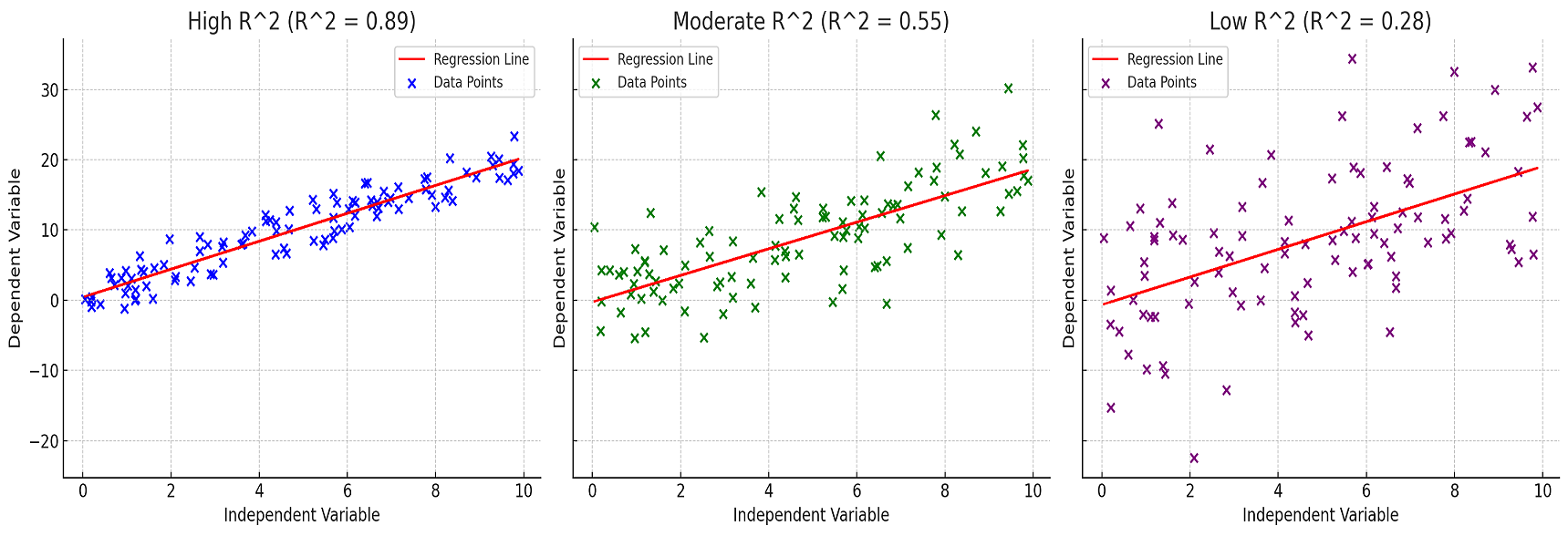
The plots above visually represent three different scenarios of R-squared in linear regression:
-
High R-squared (Left Plot):
- The data points (blue) are closely aligned with the regression line (red).
- This indicates a strong linear relationship between the independent and dependent variables.
- The R-squared value is high (close to 1), suggesting that the model explains a significant proportion of the variance in the dependent variable.
-
Moderate R-squared (Middle Plot):
- Here, the data points (green) show more dispersion around the regression line.
- The linear relationship is still evident but not as strong as in the high R-squared scenario.
- The R-squared value is moderate, indicating that the model explains a decent but not overwhelming portion of the variance.
-
Low R-squared (Right Plot):
- The data points (purple) are widely scattered around the regression line.
- This indicates a weak linear relationship between the variables.
- The low R-squared value suggests that the model does not explain much of the variance in the dependent variable.
Mathematical Explanation of R-Squared
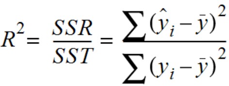
Mathematically, it can be determined as a ratio of total variation of data points explained by the regression line (Sum of squared regression) and total variation of data points from the mean (also termed as sum of squares total or total sum of squares). The following formula represents the ratio. y_hat represents the prediction or a point on the regression line, y_bar represents the mean of all the values and y_i represents the actual values or the points.
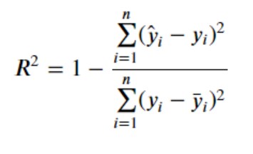
It can also be calculated as a function of total variation of data points from the regression line (also termed as sum of square residual) and total variation of data points from the mean. The following represents the formula. y_hat represents the prediction or a point on the regression line, y_i represents the actual values or the points and y_bar represents the mean of all the values
Let’s understand the concepts and formulas in detail. Once we have built a multilinear regression model, the next thing is to determine the model performance. The model predictability performance can be evaluated in terms of R-squared or coefficient of determination, although the more suitable measure is adjusted R-squared. The concepts of adjusted R-squared and how it is different from R-squared will be dealt in another blog. Let’s look at the following diagram to understand the concepts of R-squared.
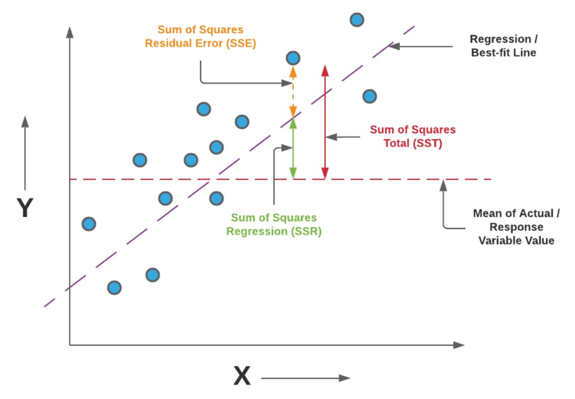
Note some of the following in the above diagram in relation to learning the concepts of R-squared / R2.
- The horizontal red line represents the mean of all the values of the response variable of the regression model. In the diagram, it is represented as mean of actual / response variable value.
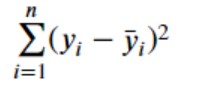
- The variation of the actual values from the mean or the horizontal line is represented as a function of variance of the points from the mean. Thus, the variation of the values from the mean is calculated as the sum of squared distance of individual points from the mean. This is also called sum of squares total (SST). Recall that the variance (σ2) is used to measurehow data points in a specific population or sample are spread outand is calculated as the squared sum of distance of individual points from the mean divided by N or N – 1 depending upon whether the population variance or the sample variance needs to be calculated respectively. At times, SST is also referred to as the total error. Mathematically, SST is represented as the following where y_bar represents the mean value and the y_i represents the actual value.
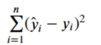
- The total variation of actual values from the regression line represents the prediction error in terms of sum of squared distance between the actual values and the prediction made by regression line. It is also termed as sum of squared residuals error (SSE). Mathematically, SSE is represented as the following where y_hat represents the prediction and the y_i represents the actual value.
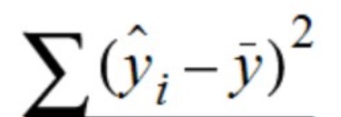
- The total variation of prediction (represented using regression line) from the mean is represented as sum of squared distance between the prediction and the mean. It is also termed as sum of squared regression (SSR). At times, the SSR is also termed as the explained error or explained variance. Mathematically, SSR is represented as the following where y_hat represents the prediction and the y_bar represents the mean value.
R-Squared Concepts & Best-fit Regression Line
The following are important concepts to be understood in relation to the value of R-squared and how is it used to determine the best-fit line or regression model performance.
- Greater the value of SSR or sum of squared regression, better is the regression line. In other words, closer the value of SSR to SST (sum of squared total), better is the regression line. That would mean the value of R-squared to be closer to 1 as R-squared = SSR / SST
- Lesser the value of SSE of sum of squared residuals, better is the regression line. In other words, closer the value of SSE to zero (0), better is the regression line. That would mean that the value of R–squared is closer to 1 as R-squared = 1 – (SSE/SST).
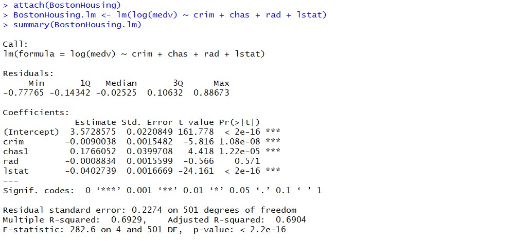
When you fit the linear regression model using R programming, the following gets printed out as summary of regression model. Note the value of R-squared as 0.6929. We can look for more predictor variables in order to appropriately increase the value of R-squared and adjusted R-squared. The data below represents the regression model built to predict the housing price in terms of predictor variables such as crim, chas, rad, lstat. You can load the BostonHousing data as part of mlbench package in R.
R-Squared for Regression Models: Python Code Example
In this section, we will look into Python code example that demonstrates how to use R-squared in the context of linear regression. In this example, we’ll:
- Fit a linear regression model to the data.
- Calculate the R-squared value to assess the model’s performance.
import numpy as np
from sklearn.linear_model import LinearRegression
from sklearn.metrics import r2_score
import matplotlib.pyplot as plt

# Generate synthetic data
#
np.random.seed(0)
x = np.random.rand(100, 1) * 10  # Independent variable
y = 2 * x + np.random.randn(100, 1) * 2  # Dependent variable with some noise

# Fit Regression Model
#
model = LinearRegression()
model.fit(x, y)

# Predict and calculate R-squared
#
y_pred = model.predict(x)
r2 = r2_score(y, y_pred)

# Plotting the results
#
plt.scatter(x, y, color='blue', label='Data Points')
plt.plot(x, y_pred, color='red', label='Regression Line')
plt.title(f'R-squared: {r2:.2f}')
plt.xlabel('Independent Variable')
plt.ylabel('Dependent Variable')
plt.legend()
plt.show()
Here is the plot representing regression model for a specific R-squared value.
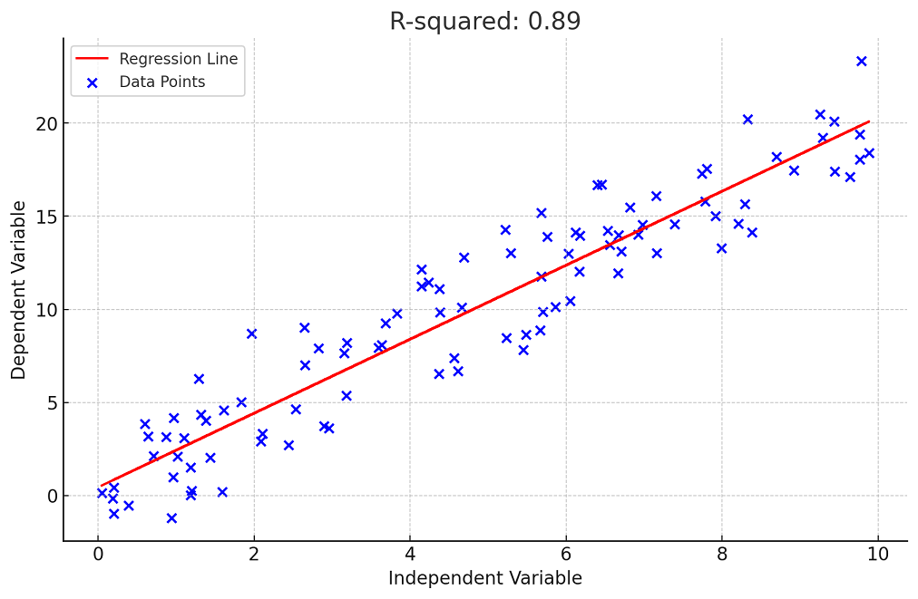
The executed Python code produces a scatter plot that visualizes the linear regression model’s fit to the synthetic data. Here’s a breakdown of the result:
- Data Points (Blue Dots): Represent the synthetic data generated for the independent variable (X-axis) and the dependent variable (Y-axis). The dependent variable has been constructed to have a linear relationship with the independent variable, plus some random noise.
- Regression Line (Red Line): This is the line of best fit determined by the linear regression model. It represents the model’s prediction of the dependent variable based on the independent variable.
Summary
In this post, you learned about the concept of R-Squared and how it is used to determine how well the multilinear regression model fit the data. The value of R-Squared lies in the range of 0 and 1. Closer the value of R-Squared to 1, better is the regression model. The value of R-Squared increases with the addition of features. However, one should consider the value of adjusted R-Squared for deciding whether to add the features or not. The concept of adjusted R-squared will be dealt in the next blog.

Check out my latest book titled as First Principles Thinking: Building winning products using first principles thinking.
- Three Approaches to Creating AI Agents: Code Examples - June 27, 2025
- What is Embodied AI? Explained with Examples - May 11, 2025
- Retrieval Augmented Generation (RAG) & LLM: Examples - February 15, 2025
I found it very helpful. However the differences are not too understandable for me