Linear regression is a foundational algorithm in machine learning and statistics, used for predicting numerical values based on input data. Understanding the cost function in linear regression is crucial for grasping how these models are trained and optimized. In this blog, we will understand different aspects of cost function used in linear regression including how it does help in building a regression model having high performance.
What is a Cost Function in Linear Regression?
In linear regression, the cost function quantifies the error between predicted values and actual data points. It is a measure of how far off a linear model’s predictions are from the actual values. The most commonly used cost function in linear regression is the Mean Squared Error (MSE) function. The MSE function is defined as:
$MSE = \frac{1}{n} \sum_{i=1}^{n} (y_i – \hat{y}_i)^2$
Where:
- n is the number of data points
- $y_i$ is the actual value
- $y^i$ is the predicted value
Implementing Linear Regression Cost Function using Python
Let’s look into an example of how do we calculate cost function value in linear regression using Python. In the following code, we have a dataset and a simple linear model with pre-determined value of coefficient (theta1) and bias (theta0). The cost function is calculated using the code mse = np.mean((Y – Y_pred) ** 2). This function computes the average of the squared differences between the actual values and the predicted values, giving a single numerical value (the MSE) that represents the average error of the model. This is the Mean Squared Error, a common metric used to evaluate the performance of a regression model.
import numpy as np

# Sample data
X = np.array([1, 2, 3, 4, 5])  # Input features
Y = np.array([2, 4, 5, 4, 5])  # Actual output

# Assuming a simple linear model with weights
theta0 = 0.5
theta1 = 0.9

# Predicted values
Y_pred = theta0 + theta1 * X

# Calculating MSE
mse = np.mean((Y - Y_pred) ** 2)
print("MSE:", mse)
Determining the values of theta1 ($theta_1$) and theta0 ($theta_0$) in linear regression is a key part of the model training process. These parameters represent the intercept and slope of the line that best fits the data, respectively. The process of finding these values is known as linear regression model fitting, and it aims to minimize the cost function, typically the Mean Squared Error (MSE).
Why & how do we minimize Cost Function in Linear Regression?
Here is the most common and popular method to determine the optimal parameter values of linear regression models by minimizing the cost function:
Gradient Descent
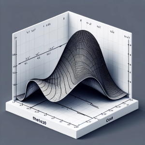
Gradient Descent is the most common method used for finding the optimal values of $theta_0$ and $theta_1$. In case of multiple linear regression model, it would be $theta_0$, $theta_1$, $theta_2$, …, $theta_n$. It’s an iterative optimization algorithm used to minimize the cost function. During the training process, Gradient Descent uses the cost function to determine how far off the model’s predictions are from the actual values and which direction the parameters should be adjusted to reduce this error. The process continues iteratively, adjusting the model parameters slightly in each step to minimize the cost function until it converges to a minimum value or until a certain number of iterations are completed.
Here’s a simplified overview of how it works for simple linear regression model:
- Initialize $theta_0$ and $theta_1$ with random values.
- Calculate the gradient of the cost function with respect to each parameter. This tells us the direction to move in the parameter space to decrease the cost function.
- Update $theta_0$ and $theta_1$ by moving them a small step in the direction that reduces the cost function. The size of the step is determined by the learning rate.
- Repeat the process until the cost function converges to a minimum.
What’s a Good Value of Cost Function in Linear Regression?
Determining a “good” value for the cost function in linear regression, such as Mean Squared Error (MSE), is not straightforward because it greatly depends on the context of the data and the specific problem being addressed. However, there are some guidelines and considerations that can help in assessing whether the cost function value is acceptable:
- Context of Data: A good MSE value is relative to the scale of your target variable. For instance, an MSE of 5 might be small if the target values range in the thousands, but it could be considered large if your target values range around 10.
- Baseline Comparisons: Compare your model’s MSE to a baseline model, such as a simple average or a historical model. If your model’s MSE is significantly lower than that of the baseline, it can be considered an improvement.
- Relative Improvement: For iterative models, such as those tuned during machine learning, a good MSE value is one that shows improvement over previous iterations. In other words, it refers to the process of model training and optimization in machine learning, particularly in the context of iterative algorithms like gradient descent. A key goal of training is to minimize the MSE. So, a “good” MSE value in one iteration is one that is lower than the MSE value from the previous iteration. This indicates that the model is getting better at making predictions – the errors between the predicted values and the actual values are, on average, becoming smaller.
- Domain-Specific Benchmarks: Different domains may have different acceptable thresholds for MSE. For example, in high-stakes fields like finance or healthcare, a lower MSE might be crucial compared to less critical applications.
- Distribution of Errors: In addition to the value of MSE, it’s also important to examine the distribution of errors. A model might have a low MSE but could be consistently under or over-predicting in certain areas.
- Compare with Variance of Data: If the MSE is significantly lower than the variance of the target variable, it usually indicates a good fit.

Check out my latest book titled as First Principles Thinking: Building winning products using first principles thinking.
- Three Approaches to Creating AI Agents: Code Examples - June 27, 2025
- What is Embodied AI? Explained with Examples - May 11, 2025
- Retrieval Augmented Generation (RAG) & LLM: Examples - February 15, 2025
I found it very helpful. However the differences are not too understandable for me