Hierarchical clustering a type of unsupervised machine learning algorithm that stands out for its unique approach to grouping data points. Unlike its counterparts, such as k-means, it doesn’t require the predetermined number of clusters. This feature alone makes it an invaluable method for exploratory data analysis, where the true nature of data is often hidden and waiting to be discovered. But the capabilities of hierarchical clustering go far beyond just flexibility. It builds a tree-like structure, a dendrogram, offering insights into the data’s relationships and similarities, which is more than just clustering—it’s about understanding the story your data wants to tell.
In this blog, we’ll explore the key features that set hierarchical clustering apart, delve into its types (agglomerative and divisive), and discuss its wide array of application. You will learn about the concepts of Hierarchical clustering with the help of Python code example. As data scientist / machine learning enthusiasts, you would want to learn the concepts of hierarchical clustering in a great manner.
What is Hierarchical Clustering?
Hierarchical clustering is Hierarchical clustering is a type of unsupervised machine learning algorithm used to group similar objects into clusters. Unlike many other clustering methods, such as k-means, hierarchical clustering does not require you to specify the number of clusters beforehand. Instead, it builds a hierarchy of clusters either by successively merging smaller clusters into larger ones (agglomerative approach) or by splitting larger clusters into smaller ones (divisive approach).
Unique Features of Hierarchical Clustering
The following are some of the unique features of hierarchical clustering:
- Hierarchical Structure: The algorithm builds a tree-like structure (dendrogram) that shows the arrangement of the clusters and their proximity. This structure can be insightful for understanding the data’s similarities and relationships. The following diagram
- No Need to Specify Number of Clusters: Unlike k-means, hierarchical clustering doesn’t require the number of clusters to be defined a priori. This can be particularly useful when the number of natural groupings is not known.
- Flexibility in Distance Metrics: Hierarchical clustering can work with different distance/similarity metrics (like Euclidean distance, Manhattan distance, cosine similarity), and different linkage criteria (like single linkage, complete linkage, average linkage) which determine how the distance between clusters is measured.
The hierarchical clustering can be classified into the following two different type of clustering:
- Agglomerative (bottom-up) hierarchical clustering: Starts by treating each data point as a single cluster and then successively merges the closest pairs of clusters until all the points are merged into a single cluster.
- Divisive (top-down) hierarchical clustering: Starts with all data points in a single cluster and recursively splits the most heterogeneous cluster until each data point is in its own cluster.
Agglomerative (Bottom-up) Hierarchical Clustering
In agglomerative clustering, the cluster formation starts with individual points. Each point is considered as one cluster. Let’s say there are N data points. In the beginning, there will be N clusters. Then, the distance between each pair of cluster is found and the clusters closest to each other is matched and made as one cluster. This would result in (N – 1) cluster. In the next step, the distance between pair of clusters are found and the clusters closest to each other is matched and made as one cluster. This would result in (N – 2) clusters. The same process is repeated until all the data points are merged into one cluster. e.g., root cluster.
It is also called as bottom-up hierarchical clustering as the clustering process starts with individual data point and move further up to form one cluster – root cluster. In the diagram below, note as to how the clusters have been formed starting from the leaf node and moving upward.
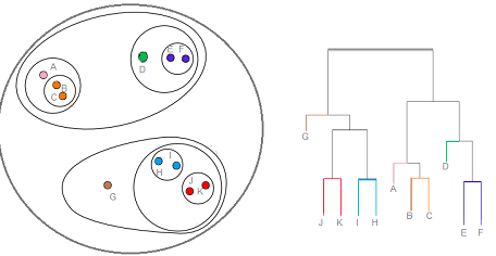
In the above diagram, on the right hand side of the picture is what is called as Dendogram. In the beginning, all of the members (letter A – G) are in the leaf node.
- In first step, cluster of J/K, I/H, B/C and E/F are formed.
- In step 2, A and cluster B/C are joined to form one cluster.
- In step 3, D is joined with cluster E & F to form a cluster.
- In step 4, Cluster J/K and I/H are joined to form one cluster.
- In step 5, G is joined with cluster in step 4 to form one cluster.
- In step 6, cluster formed in step 2 and step 3 are joined to form one cluster.
- In last step, the cluster formed in step 5 and 6 are joined to form the root cluster.
The node of the Dendogram represents the subset of points. Cutting the Dendogram at different levels will give different number of clusters. Thus, if one cut the Dendogram after first level, one will get the four clusters (J/K, I/H, B/C and E/F). However, if one cuts the Dendogram one level up, one will get 5 clusters such as J/K, I/H, A & B/C, D, E/F. Let’s understand the formation of cluster by slicing the Dendogram at any specific level using the following diagram.
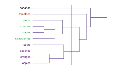
In the above Dendogram diagram, slicing vertically with red line results in creation of four clusters using different color codes.
The agglomerative hierarchical clustering algorithm differs based on the distance method used to create clusters. The following are common distance methods used to create clusters:
- Single link: Distance between the cluster is determined based on the distance between most similar two points in the two clusters. In other words, the nearest two points distance in two cluster is used to determine the cluster distance.
- Complete link: Distance between the cluster is determined based on the distance between least similar two points in the two clusters. In other words, the farthest two points distance in two cluster is used to determine the cluster distance.
- Centroid: Distance between the cluster is determined based on the distance between the centroid of the two clusters.
- Average link: Distance between the cluster is determined based on the average distance between all points in the two clusters.
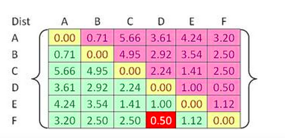
The clustering method makes use of one of the above distance calculation methods and a distance matrix such as the following to determine the cluster. Note how the distance between point D & F is smallest and thus, D & F can be made as one cluster.
Divisive (Top-down) Hierarchical Clustering
In divisive hierarchical clustering, the cluster formation starts with all the points being formed as one cluster. Applying K-means clustering in recursive manner can result in multiple clusters formation in divisive manner resulting in set of clusters with one individual points. The following represents the divisive hierarchical clustering algorithm:
- First and foremost, all points form part of root cluster.
- The root cluster is divided into two clusters, say, cluster A and B by using K-means clustering
- Each of the clusters (A & B) in previous step will be further divided into two clusters each using K-means. This would result in four clusters overall.
- Same step as above will be followed until cluster having individual points are formed.
Lets understand the algorithm using the diagram shown below:
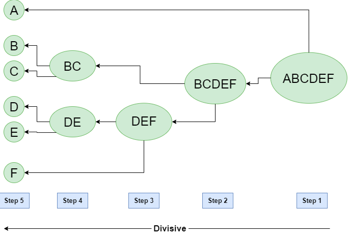
In the diagram shown above, the clustering starts with the root cluster having points A, B, C, D, E. This results in two clusters such as A and BCDEF. Applying clustering on BCDEF results in another two clusters such as BC and DEF. This process continues until there are clusters with individual points.
Hierarchical Clustering Python Example
Here is the Python Sklearn code which demonstrates Agglomerative clustering. Pay attention to some of the following which plots the Dendogram. Dendogram is used to decide on number of clusters based on distance of horizontal line (distance) at each level. The number of clusters chosen is 2.
import numpy as np
import pandas as pd
from sklearn.preprocessing import StandardScaler, normalize
from sklearn.decomposition import PCA
import scipy.cluster.hierarchy as hc
import matplotlib.pyplot as plt
from sklearn.cluster import AgglomerativeClustering
#
# Load the CSV file
#
df = pd.read_csv("/Users/apple/Downloads/cc_general.csv")
#
# Drop the customer id column
#
df = df.drop('CUST_ID', axis = 1)
#
# Fill the missing values with ffill method
#
df.fillna(method ='ffill', inplace = True)
#
# Scale the data and normalize
#
sc = StandardScaler()
df_scaled = sc.fit_transform(df)
df_normalized = normalize(df_scaled)
#
# Reduce the dimensionality of data to 3 features
#
pca = PCA(n_components=3)
df_pca = pca.fit_transform(df_normalized)
df_pca = pd.DataFrame(df_pca)
df_pca.columns = ['P1', 'P2', 'P3']
#
# Create the Dendogram plot
#
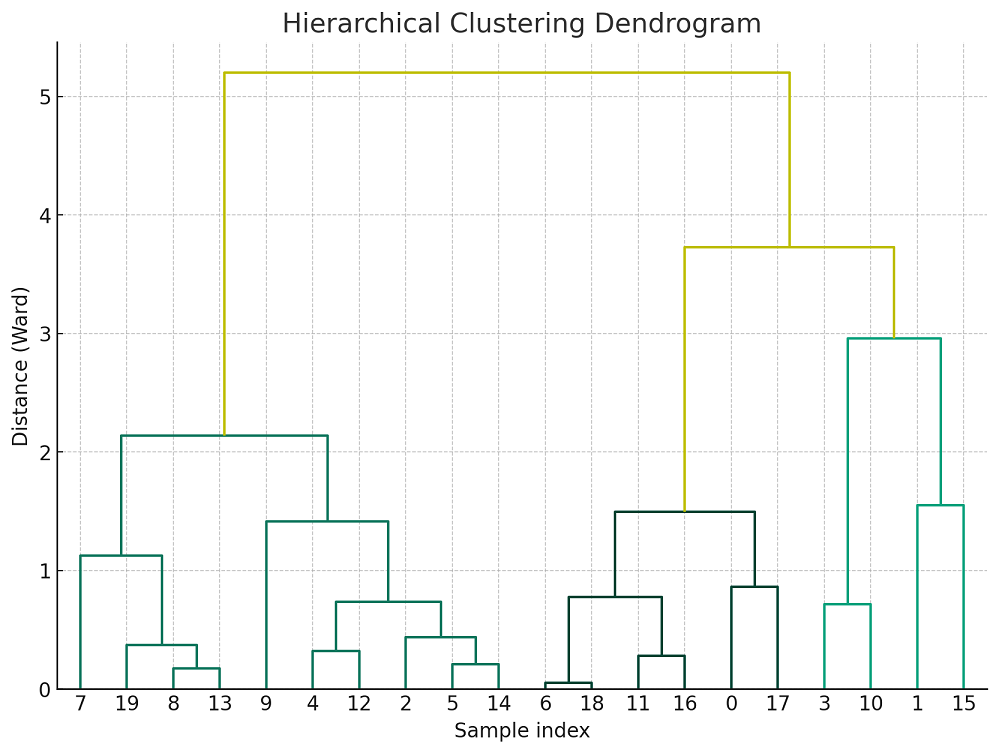
plt.figure(figsize =(8, 8))
plt.title('Visualising the data')
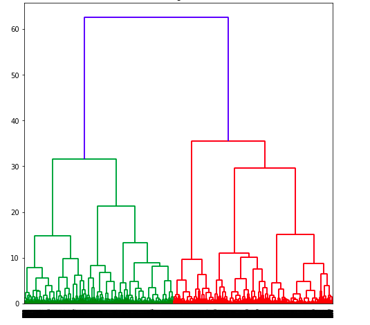
dendrogram = hc.dendrogram((hc.linkage(df_pca, method ='ward')))
The following Dendogram plot is created.
Based on the above dendogram, lets select different number of clusters and create plot based on slicing the dendogram at different levels. The picture below represents the slicing of Dendogram at four different levels and coming up different number of clusters.
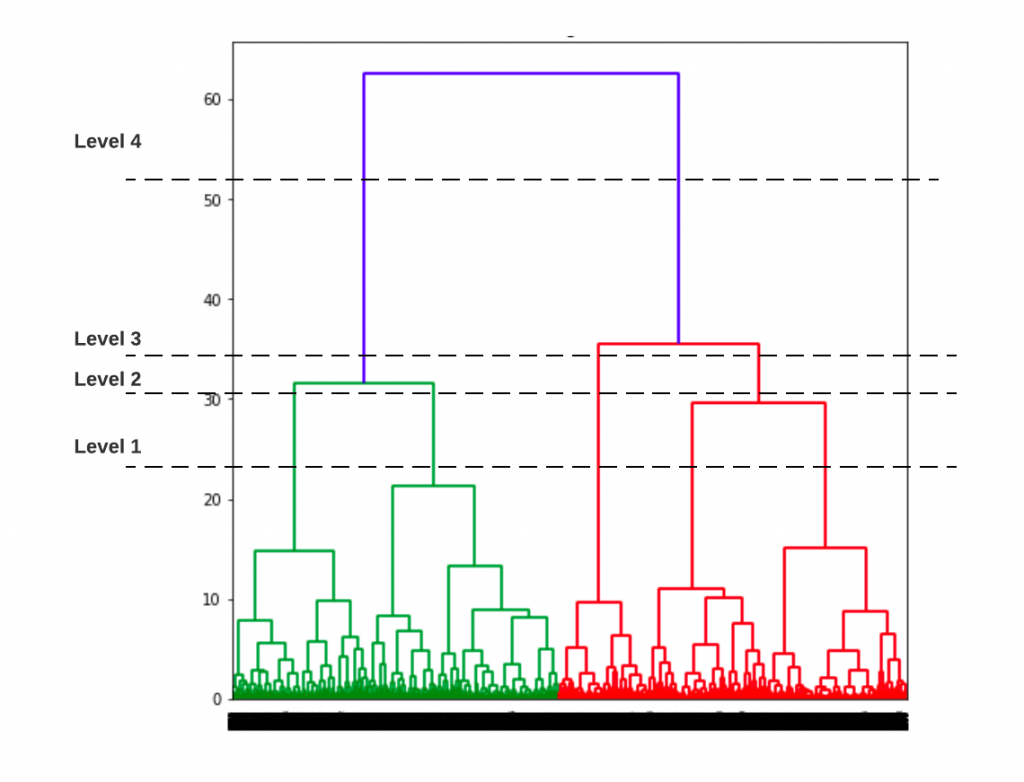
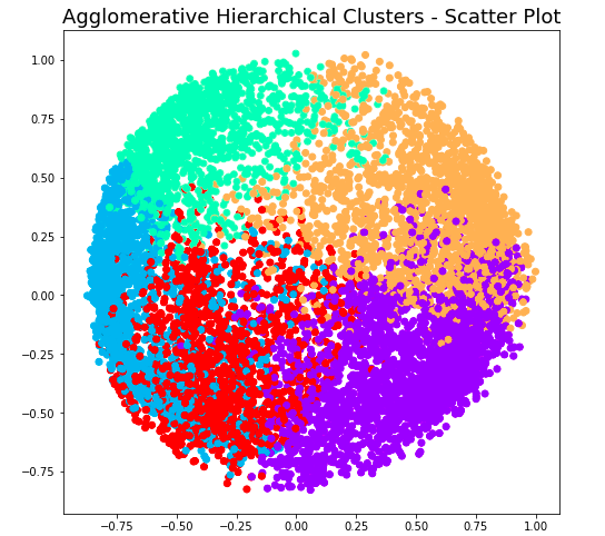
At level 1, note that there will be 5 clusters. Here is the code and related plot.
#
# Create the clusters using Agglomerative hierarchical clustering
#
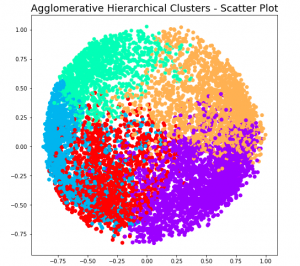
agc = AgglomerativeClustering(n_clusters = 5)
plt.figure(figsize =(8, 8))
plt.scatter(df_pca['P1'], df_pca['P2'], c = agc.fit_predict(df_pca), cmap ='rainbow')
plt.title("Agglomerative Hierarchical Clusters - Scatter Plot", fontsize=18)
plt.show()
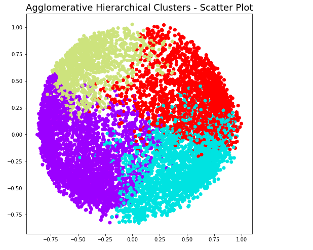
At level 2, note that there will be 4 clusters. Here is the code and related plot.
#
# Create the clusters using Agglomerative hierarchical clustering
#
agc = AgglomerativeClustering(n_clusters = 4)
plt.figure(figsize =(8, 8))
plt.scatter(df_pca['P1'], df_pca['P2'], c = agc.fit_predict(df_pca), cmap ='rainbow')
plt.title("Agglomerative Hierarchical Clusters - Scatter Plot", fontsize=18)
plt.show()
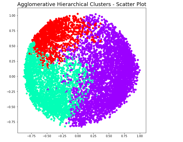
At level 3, note that there will be 3 clusters. Here is the code and related plot.
#
# Create the clusters using Agglomerative hierarchical clustering
#
agc = AgglomerativeClustering(n_clusters = 3)
plt.figure(figsize =(8, 8))
plt.scatter(df_pca['P1'], df_pca['P2'], c = agc.fit_predict(df_pca), cmap ='rainbow')
plt.title("Agglomerative Hierarchical Clusters - Scatter Plot", fontsize=18)
plt.show()
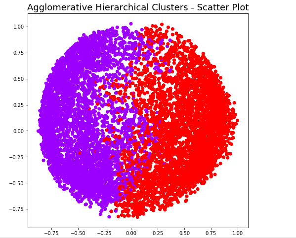
At level 4, note that there will be 2 clusters. Here is the code and related plot.
#
# Create the clusters using Agglomerative hierarchical clustering
#
agc = AgglomerativeClustering(n_clusters = 3)
plt.figure(figsize =(8, 8))
plt.scatter(df_pca['P1'], df_pca['P2'], c = agc.fit_predict(df_pca), cmap ='rainbow')
plt.title("Agglomerative Hierarchical Clusters - Scatter Plot", fontsize=18)
plt.show()
Conclusions
Here is the summary of what you learned in this post related to Hierarchical clustering:
- Hierarchical clustering is an unsupervised learning algorithm used to create the clusters based on hierarchical ordering
- There are two different types of hierarchical clustering algorithm – Agglomerative clustering and Divisive clustering
- In agglomerative hierarchical clustering, clustering starts from individual points and clusters are formed upward until one cluster – root cluster remains. It is also called as bottom-up hierarchical clustering.
- In divisive hierarchical clustering, clustering starts from the top, e..g., entire data is taken as one cluster. Root cluster is split into two clusters and each of the two is further split into two and this is recursively continued until clusters with individual points are formed. It is also called as top-down hierarchical clustering.

Check out my latest book titled as First Principles Thinking: Building winning products using first principles thinking.
- Mathematics Topics for Machine Learning Beginners - July 6, 2025
- Questions to Ask When Thinking Like a Product Leader - July 3, 2025
- Three Approaches to Creating AI Agents: Code Examples - June 27, 2025
I found it very helpful. However the differences are not too understandable for me