Last updated: 26th August, 2024
In this blog post, we will discuss the concepts of logistic regression machine learning algorithm with the help of python example. Logistic regression is a parametric algorithm which is used to estimate the probability of an event occurring. For example, it can be used in the medical field to predict the probability of a patient developing a certain disease based on various health indicators, such as age, weight, and blood pressure. It is often used in machine learning applications.
What is Logistic Regression?
Logistic regression is a type of supervised learning classification algorithm that is adept not only in binary classification but also in multinomial classification problems. It can predict whether an instance belongs to one of multiple classes. For example, a logistic regression model can be employed to determine the probability that a given sample belongs to one of two or more possible classes. It might determine, for example, that there’s a 10% chance the values in a sample correspond to class 0 and a 90% chance they correspond to class 1. In this case, logistic regression will predict that the sample corresponds to class 1.
Logistic regression model effectively learns the relationship between input features and their corresponding class labels. Unlike linear regression which maps inputs to continuous outputs, the logistic regression algorithm maps inputs to probabilities. Check more details on this blog – Linear Regression vs Logistic Regression.
In binary classification, logistic regression maps input data to a probability between 0 and 1, indicating the likelihood of one of two possible outcomes. In the context of multinomial classification, the logistic regression algorithm extends this approach to accommodate multiple classes, assigning probabilities to each class for a given input.
Different Types of Logistic Regression
There are primarily three types of logistic regression, each tailored for different kinds of classification problems:
-
Binary Logistic Regression: This is the most common form of logistic regression, used when the target variable has two possible outcomes. It predicts the probability that an instance belongs to each of the two categories. For example, determining whether an email is spam or not spam is a binary classification problem.
-
Multinomial Logistic Regression: This type is used when the target variable can fall into more than two categories that are not ordered. It is suitable for scenarios where the outcome needs to be categorized into three or more classes in no specific order. For instance, predicting the type of cuisine a restaurant serves (like Italian, Chinese, Indian, etc.) based on various features would be a multinomial logistic regression problem.
-
Ordinal Logistic Regression: This variant is used when the target variable has three or more ordinal categories. In this case, the categories have a natural order, but the intervals between the categories are not necessarily consistent. For example, rating satisfaction levels as ‘satisfied’, ‘neutral’, or ‘dissatisfied’ would be an appropriate application for ordinal logistic regression.
Each type of logistic regression applies the logistic or sigmoid function to model the probability of class membership based on one or more predictor variables. The choice of which type to use depends on the nature of the target variable in the dataset.
How does Logistic Regression work?
In logistic regression, the core operation is transforming input data into a probability value, which is achieved using the sigmoid function. The “why” behind this process is rooted in the goal of logistic regression: to predict the probability of a binary outcome (yes/no, true/false, 1/0). Unlike linear regression which outputs continuous values, logistic regression is used when the output is categorical. The output in logistic regression needs to represent a probability that a sample belongs to each of the classes.
The sigmoid function, also known as the logistic function, is a special mathematical equation that transforms any real-valued number into a value between 0 and 1. It’s given by:
$$\Large \sigma(z) = \frac{1}{1 + e^{-z}} $$ …(eq. 1)
The value of z in sigmoid function represents the weighted sum of input values and can be written as the following:
$$\Large z = \theta^{T}x $$ …(eq. 2)
Where θ represents the parameters.
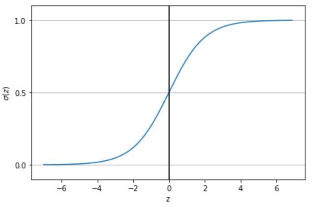
The sigmoid function, plotted (below) against its input z, illustrates how smoothly transitions from 0 to 1. As increases, it approaches 1, and as decreases towards negative infinity, gets closer to 0. Notably, at , is exactly 0.5.
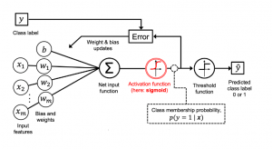
The picture below represents different aspects of a logistic regression model:
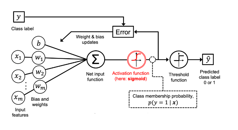
Based on the above picture, the following represents some of the key concepts related to logistic regression model:
- A set of input features ($x_i$) and related weights ($w_i$) combines together and get added to the bias element (b). This is depicted as new input function in the above diagram. This is same as linear regression function. It is same as “z” shown in equation 1 of the above formula. This is in line with the fact that logistic regression is a parametric model.
- The net input is passed to the sigmoid function and the output of the sigmoid function ranges from 0 to 1
- The output of $ \sigma(z) $ = P(Y = 1| x; w, b). The output represents the probability that a particular data point or example would belong to class 1 given its features x with parameters as weights (w) and the bias (b). Taking the example of IRIS data set, if the goal is to predict whether a flower is IRIS-Versicolor and the value of $ \sigma(z) $ = 0.75. This means that the probability that the data points belong to the flower Versicolor is 0.75. When keeping the threshold as 0.5, we can predict that the flower is Versicolor. The predicted probability can be converted to the binary outcome of class 1 or 0 (Versicolor or otherwise in this example) can be represented via the following threshold function.
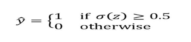 The threshold function will become like the following as a function of z (summation of weights and features added with the bias). Refer the sigmoid plot above. For the value of z greater than or equal to 0, one can predict the outcome to be class 1.
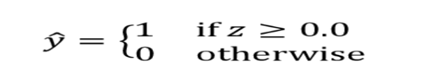
- The output from sigmoid function is passed to a threshold function (as shown above) which then sends output as 1 or 0, 1 for the positive class.
- The logistic regression model’s decision boundary is critical – it’s the threshold used to determine the class label. This decision boundary can be set to values other than 0.5, depending on the specific problem.


The output of the logistic regression model (sigmoid function output) is always between 0 and 1. For a binary classification model, if the output is close to 0, it means that the event is less likely to occur. If the output is close to 1, it means that the event is more likely to happen. For example, if the value of logistic regression model (represented using sigmoid function) is 0.8, it represents that the probability that the event will occur is 0.8 given a particular set of parameters learned using cost function optimization. Based on the threshold function, the class label can said to be 1. For any new value X, the output of the above function will be used for making the prediction.
Logistic Regression Model Parameters – How to Estimate?
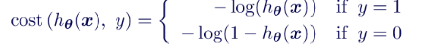
The parameters in logistic regression is learned using the maximum likelihood estimation. The cost function for logistic regression is defined as:

In above cost function, h represents the output of sigmoid function shown earlier, y represents the class/label of the training data, x represents the training data. Note that for binary classification problems, the first term will be zero for class labeled as as 0 and the second term will be zero for class labeled as 1. The equation below represents this aspect:
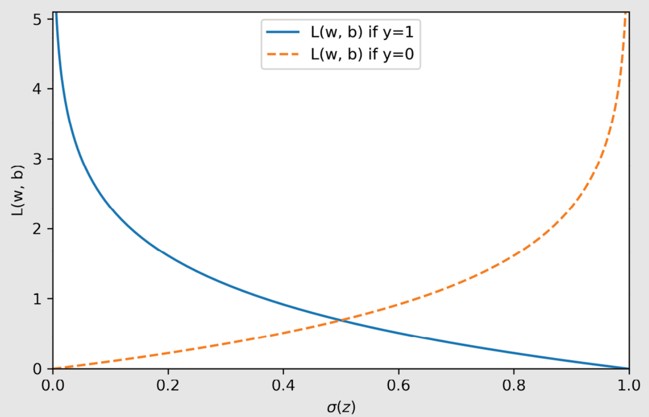
When the loss function is plotted against hypothesis function (sigmoid), the following plot occurs for y = 0 and y = 1.
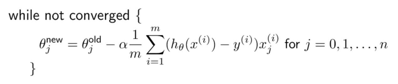
In order to fit the parameters, the objective function J(θ) would need to be minimized. Gradient descent algorithm (stochastic gradient descent – SGD) can be used for optimizing the objective or cost function. This is how the equation looks like for updating the parameters when executing gradient descent algorithm. Ensuring that gradient descent is running correctly, the value of J(θ) is calculated for θ and checked that it is decreasing on every iteration.
Besides stochastic gradient descent algorithm, it is recommended to use advanced algorithms such as some of the following: Conjugate gradient, BFGS, L-BFGS etc. When using scikit-learn for training logistic regression models, these algorithms can be used by mentioning solver parameter such as newton-cg, lbfgs, liblinear, saga, sag, etc.
Check out my video on cost function of the logistic regression model to learn the details.
Logistic Regression Applications / Examples
The following represents few examples of problems that can be solved using binary classification model trained using logistic regression algorithm:
- Spam email classification: In the context of spam email classification, logistic regression can be used to determine whether an email is spam or not. The algorithm does this by training on a dataset of labeled emails (i.e., emails that have been manually classified as spam or not spam). Once the algorithm has been trained, it can then be applied to new emails to make predictions about their labels. When training the logistic regression model for spam email classification because a variety of features of an email (such as the presence of certain keywords) is considered in order to make its predictions.
- Fraudulent online transactions: In the context of online fraud detection, logistic regression can be used to classify transactions as either fraudulent or not fraudulent. This is done by inputting a variety of factors into the regression model, such as the amount of money involved in the transaction, the method of payment, the shipping address, etc. By analyzing this data, the model can generate a prediction about whether the transaction is likely to be fraudulent. This information can then be used by businesses to help prevent losses due to fraud.
- Loan default: Logistic regression models can be used to predict whether a loan will default. It does this by assigning a probability to each loan, based on factors such as the borrower’s credit score, employment history, loan amount, etc. The Logistic regression algorithm then uses these probabilities to classify loans into two groups: those that are likely to default, and those that are not. Logistic regression models are powerful in the sense that they can help lenders to identify loans that are more likely to default. This information can be used to make better decisions about which loans to approve and how to price them. Logistic regression can also be used to develop strategies for managing loan portfolios. For example, the model can be used to identify which loans are more likely to become delinquent and how to allocate resources to minimize losses.
- Malignant tumor: In the context of tumors, logistic regression can be used to classify tumors as benign or malignant. This is a important task, as it can help doctors to make treatment decisions. There are a number of factors that can be used to classify tumors, including size, shape, and texture.
Logistic Regression Model Python Example
The Python code used in this blog represents fitting a machine learning model using Logistic Regression (Sklearn Logistic Regression). First and foremost, we will load the appropriate packages, sklearn modules and classes.
# Importing basic packages
#
import numpy as np
import pandas as pd
import matplotlib.pyplot as plt

# Importing Sklearn module and classes
from sklearn.linear_model import LogisticRegression
from sklearn.preprocessing import StandardScaler
from sklearn import metrics
from sklearn import datasets
from sklearn.model_selection import train_test_split
Data Loading – IRIS dataset
The IRIS data set is used for training the logistic regression model. The Iris data set is a classification dataset that contains three classes of 50 instances each, where each class refers to a type of iris plant. The three classes in the Iris dataset are:
- Setosa
- Versicolor
- Virginica
As a next step, we will load the dataset and do the data preparation. The scikit-learn library will be used to load the Iris dataset.
iris = datasets.load_iris()
X = iris.data[:, [0, 2]]
Y = iris.target
Create Training / Test Data
Next step is to create a train and test split. Note the stratification parameter. This is used to ensure that class distribution in training / test split remains consistent / balanced.
X_train, X_test, Y_train, Y_test = train_test_split(X, Y, test_size=0.3, random_state=1, stratify=Y)
Perform Feature Scaling
Next step is to perform feature scaling in order to make sure features are in fixed range irrespective of their values / units etc.
sc = StandardScaler()
sc.fit(X_train)
X_train_std = sc.transform(X_train)
X_test_std = sc.transform(X_test)
Train a Logistic Regression Model
Next step is to train a logistic regression model. The following needs to be noted while using LogisticRegression algorithm sklearn.linear_model implementation:
- Usage of C parameters. Smaller values of C specify stronger regularization.
- The multi_class parameter is assigned to ‘ovr‘. It represents one-vs-rest algorithm to be used. Other option is multinomial.
- The solver parameter is assigned to ‘lbfsg‘. Other solvers which can be used are newton-cg, sag, saga, lib linear
# Create an instance of LogisticRegression classifier
lr = LogisticRegression(C=100.0, random_state=1, solver='lbfgs', multi_class='ovr')

# Fit the model
#
lr.fit(X_train_std, Y_train)

Measure Logistic Regression Model Performance
Next step is to measure the model performance of the model trained using LogisticRegression as shown above. In the code below, predict method is used to predict the class. You can also use predict_proba to compute the probabilities for each class.
# Create the predictions
#
Y_predict = lr.predict(X_test_std)

# Use metrics.accuracy_score to measure the score
print("LogisticRegression Accuracy %.3f" %metrics.accuracy_score(Y_test, Y_predict))
The score method is used to quantify the accuracy of a classification model. The score method returns the model accuracy in terms of sum of the true positives and the true negatives divided by the total number of samples.
Training Logistic Regression Models with built-in Cross Validation
In case you are working with smaller datasets, and, want to train logistic regression based on cross-validation, you could use LogisticRegressionCV class. Code such as following can be used to instantiate logistic regression class with built-in CV.
model = logisticRegressionCV(cv=5)
model.fit(x, y)

Check out my latest book titled as First Principles Thinking: Building winning products using first principles thinking.
- Mathematics Topics for Machine Learning Beginners - July 6, 2025
- Questions to Ask When Thinking Like a Product Leader - July 3, 2025
- Three Approaches to Creating AI Agents: Code Examples - June 27, 2025
I found it very helpful. However the differences are not too understandable for me