
Maximum Likelihood Estimation (MLE) is a fundamental statistical method for estimating the parameters of a statistical model that make the observed data most probable. MLE is grounded in probability theory, providing a strong theoretical basis for parameter estimation. This is becoming more so important to learn fundamentals of MLE concepts as it is at the core of generative modeling (generative AI). Many models used in machine learning and statistics are based on MLE, including logistic regression, survival models, and various types of machine learning algorithms.
MLE is particularly important for data scientists because it underpins many of the probabilistic machine learning models that are used today. These models, which are often used to make predictions or classify data, require an understanding of probability distributions in order to be effective. By learning how to apply MLE, data scientists can better understand how these models work, and how they can be optimized for specific tasks.
In this blog, we will explore the concepts behind MLE and provide examples of how it can be used in practice. We will start with basic concepts of sample space, probability density, parametric modeling and then learn about likelihood and maximum likelihood estimation. We will also learn about how MLE is used in machine learning, before diving into the details of MLE and its applications. Whether you’re a seasoned data scientist or just starting out in the field, this blog will provide valuable insights into one of the key tools used in modern machine learning.
What is Maximum Likelihood Estimation?
The likelihood function is used to represent the probability of observing the data in sample space assuming the true data generating distribution was the model or density function parametrized by the $\theta$.
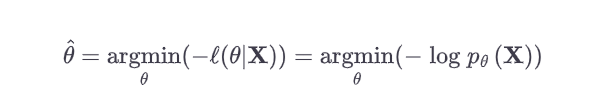
Based on the above, we learn that the goal becomes to find the optimal values of parameters of the model or density function, $\theta$ that maximizes the likelihood of seeing or observing the data (X) in the sample space. This technique or method is called as Maximum Likelihood Estimation (MLE). MLE is also used to represent maximum likelihood estimator or maximum likelihood estimate. The goal of the maximum likelihood estimation is to estimate the parameters that maximize the likelihood function. The formula below represents the maximum likelihood estimation function.

Summarizing above, the following are the core concepts that needed to be understood when learning MLE:
- Basic Idea: MLE seeks the parameter values for a model that make the observed data most probable.
- Likelihood Function: This is a function of the parameters of a statistical model, given specific observed data. For a set of parameters, it calculates the probability of observing the given data.
- Maximization: MLE finds the parameter values that maximize the likelihood function. This process involves calculus (specifically differentiation) to find the parameter values where the likelihood function peaks.
When working with neural networks, the loss function is typically minimized. Thus, we can go about finding the set of parameters that minimize the negative log-likelihood such as that given below:
Why use maximum likelihood estimation (MLE)?
The following are some of the key reasons why you would want to use MLE:
- Theoretical Foundations: MLE is grounded in probability theory, providing a strong theoretical basis for parameter estimation.
- Good Properties: Under regular conditions, MLE estimators are unbiased, consistent, and efficient.
- Versatility: MLE is applicable to a wide range of models, including linear models, generalized linear models, and even complex non-linear models.
- Asymptotic Normality: For large sample sizes, MLE estimators are approximately normally distributed, which is helpful for constructing confidence intervals and hypothesis tests.
Key concepts to learn for better understanding Maximum Likelihood Estimation (MLE)
It is recommended to learn some of the following concepts to get a holistic picture of maximum likelihood estimation (MLE) concepts:
- Sample space: Given a random variable, sample space represents all values that the random variable can take. For example, let’s consider the example of a coin toss. When a coin is tossed, there are two possible outcomes: heads or tails. These outcomes represent the sample space for this experiment. The sample space, in this case, is simply the set of all possible outcomes. It can be represented as {Heads, Tails}.
- Probability density function: Given a sample space, probability density function is a function that maps the value with a probability value between 0 and 1. The example of probability distribution function includes normal, exponential, Poisson, uniform, binomial distribution, etc.
- Parametric modeling: Parametric models represents a set of density function with one or more parameters. For different values of parameters, there will be different density function. All of these density functions can be represented as the parametric models. We can term these parameters as $\theta$. $\theta$ can be used to represent different parameters such as $\theta_1, \theta_2, \theta_3, \theta_4$, etc. For example, the probability density function of normal distribution has parameters such as mean and standard deviation. The example of parametric model can be family of density functions related to normal distribution, Poisson distribution, gamma distribution, binomial distribution, etc.
- Likelihood function: For a particular sample space, you can estimate different such parameters representing different density function. The Likelihood function represents the probability of observing or seeing the values in sample space if the true generating distribution was the model represented using the particular density function parametrized by [latex]\theta[/latex]. For a particular value x, the likelihood function is represented using the following:
$L(\theta|x) = p_{\theta}(x)$ OR, $L(\theta|x) = p(x|\theta)$
When we take into consideration the entire data in the sample space X, the likelihood function becomes the following:
$$L(\theta|x) = \prod p_{\theta}(x)$$
Given the above would result in a very small number between 0 and 1 and gets computationally difficult to work with, due to probability value for each value in sample space lying between 0 and 1, the following is recommended and often used. It is called as log likelihood function. Basically, taking log results into summation of log of output of density function for each value in sample space.

Maximum Likelihood Estimation Example: Logistic Regression
MLE underpins numerous statistical and machine learning models, encompassing logistic regression, survival analysis, and a diverse array of machine learning techniques. Let’s understand how MLE applies to logistic regression models.
Recall that logistic regression is used for modeling the probability of a binary outcome based on one or more predictor variables (features). The logistic model predicts the probability that the outcome is 1 (success) as a function of the predictors. It uses the logistic function to ensure the predicted probabilities are between 0 and 1. The logistic function is given by:
$$P(Y=1|X) = \frac{1}{1 + e^{-(\beta_0 + \beta_1 X_1 + \beta_2 X_2 + \cdots + \beta_k X_k)}}$$
Where,
- P(Y=1∣X) is the probability that the outcome Y is 1 given the predictors X.
- $\beta_0, \beta_1, \beta_2, \beta_3, …, \beta_k$ are the parameters (coefficients) of the model.
- $X_1, X_2, X_3, …, X_n$ are predictor variables.
The following is how MLE is used in logistic regression:
- Formulating the Likelihood Function:
- The likelihood function in logistic regression is the probability of observing the given set of outcomes given the predictors and the model parameters.
- For a dataset with n observations, the likelihood L is the product of individual probabilities for each observation.
- Likelihood for Each Observation:
- For an observation with outcome 1, the likelihood is (P(Y=1|X).
- For an observation with outcome 0, the likelihood is 1−P(Y=1|X).
- Overall Likelihood:
- The overall likelihood is the product of these probabilities across all observations.
- In practice, it’s more convenient to maximize the log-likelihood because products become sums, making the computation easier.
- Maximizing the Log-Likelihood:
- The MLE problem involves finding the parameter values $\beta_0, \beta_1, \beta_2, \beta_3, …, \beta_k$ that maximize the log-likelihood.
- This is typically done using numerical optimization techniques, as there is no closed-form solution for logistic regression.
- Interpreting the Parameters:
- Once the optimal parameters are found, they are used to make predictions.
- The coefficients $\beta_0, \beta_1, \beta_2, \beta_3, …, \beta_k$ represent the change in the log-odds of the outcome per unit change in the predictor variables.
In summary, MLE is central to logistic regression as it provides a systematic way to estimate the parameters that define the relationship between predictors and the probability of a binary outcome. This methodology ensures that the model is as consistent as possible with the observed data.
Conclusion
Maximum Likelihood Estimation (MLE) is a widely-used statistical method that helps us estimate the parameters of a probability density function which are used to assess the probability of observing the data in the sample space. At its core, maximum likelihood estimation is about finding the values for a set of parameters that provide the highest likelihood for the observed data. Through a variety of examples, we have explored how maximum likelihood estimation can be applied to real-world scenarios, such as predicting consumer behavior, understanding the effectiveness of medical treatments, and more. It is a powerful tool for statisticians, data scientists, and researchers that allows them to make informed decisions based on meaningful data. In short, maximum likelihood estimation is a fundamental concept in statistics that has immense practical applications in various fields, making it an essential technique to be learned and mastered by anyone interested in making data-driven decisions.

Check out my latest book titled as First Principles Thinking: Building winning products using first principles thinking.
- Mathematics Topics for Machine Learning Beginners - July 6, 2025
- Questions to Ask When Thinking Like a Product Leader - July 3, 2025
- Three Approaches to Creating AI Agents: Code Examples - June 27, 2025
I found it very helpful. However the differences are not too understandable for me