In the realm of predictive modeling and data science, regression analysis stands as a cornerstone technique. It’s essential for understanding relationships in data, forecasting trends, and making informed decisions. This guide delves into the nuances of Linear Regression and Polynomial Regression, two fundamental approaches, highlighting their practical applications with Python examples.
What are Linear and Polynomial Regression?
In this section, we will learn about what are linear and polynomial regression.
What is Linear Regression?
Linear Regression is a statistical method used in predictive analysis. It’s a straightforward approach for modeling the relationship between a dependent variable (often denoted as y) and one or more independent variables (denoted as x). In simple linear regression, there’s only one independent variable. The purpose of linear regression is to find a linear equation, y=mx+c (where m is the slope and c is the y-intercept or bias), that best fits the data. This model is extensively used in various fields like economics, biology, engineering, and more, primarily for forecasting, trend analysis, and determining causal relationships.
Expanding on this, we encounter Multiple Linear Regression, a variant that includes two or more independent variables. In this model, the equation takes the form $y = b_0 + b_1*x_1 + b_2*x_2 + … + b_n*x_n$ , where b0 is the intercept, and b1,b2,…,bn are coefficients representing the impact of each independent variable on the dependent variable. This form of regression is particularly useful in real-world scenarios where the dependent variable is influenced by multiple factors. For instance, in predicting housing prices, multiple linear regression can simultaneously account for variables like size, location, and the number of bedrooms.
The primary purpose of both simple and multiple linear regression is to find a linear function that best fits the given data.
What is Polynomial Regression?
Polynomial Regression, a more complex form of regression analysis, extends the linear model by adding extra predictors, obtained by raising each of the original predictors to a power. This model is represented as $y = a + b*x + c*x^2 + d*x^3 + …$. The purpose of polynomial regression is to capture a wider range of curvature in the data. Unlike linear regression, it’s not limited to linear relationships but can model data with non-linear trends. It’s particularly useful in cases where the relationship between the variables is not straightforward or when you need to model the fluctuations in the data more accurately.
When to Use Linear Regression and Polynomial Regression
The decision to use Linear Regression or Polynomial Regression depends on the nature of the data and the specific requirements of the analysis. Here are some guidelines to help determine when to use each:
When to Use Linear Regression
- Linear Relationship: Use linear regression when the relationship between your independent and dependent variables appears to be linear. This means that a change in the independent variable(s) results in a proportional change in the dependent variable.
- Simplicity and Interpretability: If you need a model that is easy to explain and interpret, linear regression is often preferred. Its simplicity makes it a go-to choice for situations where understanding the influence of each independent variable is crucial.
- Large Sample Size: Linear regression can be more robust to noise and overfitting, particularly with large datasets, making it suitable for analyses where you have a substantial amount of data.
- Baseline Modeling: In predictive modeling, linear regression serves as an excellent baseline. Its performance can be a benchmark for more complex models.
When to Use Polynomial Regression
- Non-linear Relationship: If the data shows a non-linear relationship, polynomial regression is more appropriate. This is particularly relevant when the change in the dependent variable does not follow a straight line but rather a curve.
- Modeling Complex Relationships: In fields like economics, environmental science, and engineering, where relationships between variables are often non-linear, polynomial regression can capture the underlying trends more effectively.
- Flexibility in Modeling Data: Polynomial regression offers greater flexibility in fitting a wide variety of curves to the data, making it suitable for datasets with complex patterns and fluctuations.
- Small to Medium-sized Datasets: Polynomial regression can fit a wider range of curves, but with smaller datasets, it’s prone to overfitting. It’s ideal for medium-sized datasets where the complexity of the model doesn’t overshadow the amount of available data.
Considerations for Both Linear and Polynomial Regression
- Overfitting vs. Underfitting: Linear regression can underfit complex datasets, while polynomial regression can overfit if the polynomial degree is too high. Balancing model complexity with the risk of overfitting is crucial.
- Data Preprocessing: Both types of regression benefit from proper data preprocessing. This includes scaling features, handling missing values, and considering interaction effects for multiple linear regression.
- Cross-validation: Regardless of the chosen model, using cross-validation techniques to assess model performance on unseen data is vital. This helps in ensuring that the model generalizes well to new data.
Evaluating Linear and Polynomial Regression Models: Suitable Metrics
When assessing models trained with Linear and Polynomial Regression, it’s important to choose evaluation metrics wisely, as some are universally applicable while others are better suited to one type of model over the other:
- Coefficient of Determination (R² Squared): Suitable for both Linear and Polynomial Regression. It measures how effectively the model explains the variance in the dependent variable. However, in Polynomial Regression, caution is needed since R² can be inflated and misleading, especially with higher-degree polynomials.
- Mean Squared Error (MSE) and Root Mean Squared Error (RMSE): Applicable to both models. These metrics assess the average error between the model’s predictions and actual values. RMSE, being the square root of MSE, provides a scale that’s easier to interpret and is sensitive to outliers.
- Mean Absolute Error (MAE): Useful for both Linear and Polynomial Regression. MAE offers a straightforward average of error magnitudes, making it a reliable measure for both types of models.
- Cross-Validation: Critical for both types. It’s a robust method to test the model’s effectiveness on unseen data, ensuring that the model generalizes well and is not overfitting, which is particularly important in Polynomial Regression.
- Residual Analysis: Important for both Linear and Polynomial Regression. This method checks whether the residuals (differences between observed and predicted values) display any patterns, indicating potential issues with the model’s fit.
- Adjusted R² Score: More relevant for Polynomial Regression. It adjusts the R² score to account for the number of predictors, making it a valuable metric for Polynomial models where the risk of overfitting is higher.
Problem Examples for Linear and Polynomial Regression
The following are real-world problems examples where linear and polynomial regression may be suitable. In each of these examples, the choice between linear and polynomial regression hinges on the nature of the relationship between the independent and dependent variables. Linear regression excels in scenarios where this relationship is straightforward and linear, while polynomial regression is better suited for more complex, non-linear relationships.
Linear Regression Examples
- Real Estate Pricing Prediction:
- Problem: Predict the selling price of houses based on features like size (square footage), location (urban/suburban), and number of bedrooms.
- Data Required: Historical data of house sales including selling prices and house features.
- Why Linear Regression: The relationship between house features and price is often linear, making linear regression suitable for a first approximation.
- Sales Forecasting for a Retail Store:
- Problem: Estimate next month’s sales based on historical sales data, taking into account factors like advertising budget, seasonality, and store location.
- Data Required: Past sales records, advertising spending, seasonal indices, and store location data.
- Why Linear Regression: It provides a straightforward model to understand how different factors linearly impact sales, aiding in budget planning and marketing strategies.
Polynomial Regression Examples
- Agricultural Yield Prediction Based on Environmental Conditions:
- Problem: Predict the crop yield based on variables such as temperature, rainfall, and soil quality, where the relationship between these factors and yield is not linear.
- Data Required: Historical data of crop yields along with corresponding environmental conditions.
- Why Polynomial Regression: Environmental factors often have a non-linear impact on crop yields. Polynomial regression can model these complex relationships more effectively than linear regression.
- Modeling Electricity Consumption in Relation to Temperature:
- Problem: Forecast the electricity consumption of a city based on the temperature, where consumption increases during extreme cold and hot temperatures but drops at moderate temperatures.
- Data Required: Historical data on electricity consumption and daily temperature records.
- Why Polynomial Regression: The relationship between temperature and electricity consumption is likely to be non-linear (U-shaped curve), making polynomial regression a better fit for capturing these dynamics.
Python Sklearn Example – Linear vs Polynomial Regression
We will illustrate the use of the sklearn module in Python for training linear and polynomial regression models with the California housing dataset.
In the Python code below, sklearn PolynomialFeatures has been used. This class can be understood as a data preprocessing tool that generates polynomial and interaction features from input data. It transforms a dataset with n features into one containing all polynomial combinations up to a specified degree, thereby enhancing the complexity and fit of regression models.
The code PolynomialFeatures(degree=2) creates an instance of the “PolynomialFeatures” class with the degree set to 2. This means it will generate all the polynomial features up to the second degree (squared terms) from the input data. The fit_transform() method first fits the PolynomialFeatures transformer to the training data and then transforms the training data into polynomial features. This includes generating interaction terms (if there are multiple features) and power terms. The transformed training data X_train_poly now contains the original features plus the additional polynomial features. Similar to the training data, X_test is reshaped and then transformed using the already fitted poly_features object. This ensures that the testing data is transformed in the same way as the training data, with the same polynomial features being generated.
Linear Regression & Polynomial Regression Python Example
import numpy as np
import pandas as pd
import matplotlib.pyplot as plt
from sklearn.datasets import fetch_california_housing
from sklearn.linear_model import LinearRegression
from sklearn.model_selection import train_test_split
from sklearn.preprocessing import PolynomialFeatures

# Load California housing dataset
california = fetch_california_housing()
X = california.data
y = california.target

# For simplicity, let's use the feature "MedInc" which is median income in block group
X_medinc = X[:, california.feature_names.index('MedInc')]

# Splitting the dataset
X_train, X_test, y_train, y_test = train_test_split(X_medinc, y, test_size=0.2, random_state=42)

# Linear Regression
lr = LinearRegression()
lr.fit(X_train.reshape(-1, 1), y_train)

# Polynomial Regression with degree 2
poly_features = PolynomialFeatures(degree=2)
X_train_poly = poly_features.fit_transform(X_train.reshape(-1, 1))
X_test_poly = poly_features.transform(X_test.reshape(-1, 1))
poly_lr = LinearRegression()
poly_lr.fit(X_train_poly, y_train)

# Predictions for plotting
x_range = np.linspace(X_medinc.min(), X_medinc.max(), 100).reshape(-1, 1)
y_lin_pred = lr.predict(x_range)
y_poly_pred = poly_lr.predict(poly_features.transform(x_range))

# Plotting
plt.figure(figsize=(10, 6))
plt.scatter(X_medinc, y, color='gray', alpha=0.5, label='Data points')
plt.plot(x_range, y_lin_pred, color='red', label='Linear Regression')
plt.plot(x_range, y_poly_pred, color='blue', label='Polynomial Regression (Degree 2)')
plt.xlabel('Median Income in Block Group')
plt.ylabel('Median House Value')
plt.title('Linear vs Polynomial Regression on California Housing Dataset')
plt.legend()
plt.show()
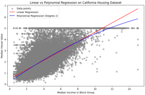
The following plot gets created. The plot displays a comparison between Linear Regression and Polynomial Regression (Degree 2) using the California Housing Dataset. The red line represents the Linear Regression model. It is a straight line that shows the average relationship between the median income and the house value. The blue line represents the Polynomial Regression model with a degree of 2. This line curves to fit the data points better than the straight line of the linear model, indicating the model is capturing some of the non-linear trends in the data.

The Polynomial Regression model appears to fit the lower and higher ends of the income scale more closely than the Linear Regression model, which could suggest a non-linear relationship in the data that the polynomial model is capturing. However, the central part of the plot (around the median income) shows both models giving similar predictions. This visualization is useful for understanding how each model approximates the underlying data distribution and can help in deciding which model might provide better predictions for the dataset at hand.

Check out my latest book titled as First Principles Thinking: Building winning products using first principles thinking.
- Questions to Ask When Thinking Like a Product Leader - July 3, 2025
- Three Approaches to Creating AI Agents: Code Examples - June 27, 2025
- What is Embodied AI? Explained with Examples - May 11, 2025
I found it very helpful. However the differences are not too understandable for me