Predicting house prices accurately is crucial in the real estate industry. However, it can be challenging to determine the factors that significantly impact house prices. Without a clear understanding of these factors, accurate predictions are difficult to achieve. The Boston Housing Dataset addresses this problem by providing a comprehensive set of variables that influence house prices in the Boston area. However, effectively utilizing this dataset and building robust predictive models require appropriate techniques and evaluation methods.
In this blog, we will provide an overview of the Boston Housing Dataset and explore linear regression, LASSO, and Ridge regression as potential models for predicting house prices. Each model has its unique properties that address specific challenges. By understanding the differences between these models, we can choose the most appropriate model for production. We will learn about how to use Mean Squared Error (MSE) for each model to evaluate their performance.
Understanding Boston Housing Dataset
Before we get into building regression models, it is important to understand the data we will be working with. In this section, we will understand the Boston Housing Dataset (https://raw.githubusercontent.com/selva86/datasets/master/BostonHousing.csv) including its structure, and, explain the meaning of each column label.
The Boston Housing Dataset is a widely used dataset in machine learning and predictive analytics. It contains housing information for various neighborhoods in Boston. This dataset contains information collected by the U.S. Census Service concerning housing in the area of Boston, Massachusetts. The dataset has 506 rows, each representing a different house in the area. There are 14 columns, each representing a different aspect of the houses and their surroundings. Following is the details of the columns:
- crim: This is the per capita crime rate by town.
- zn: This is the proportion of residential land zoned for lots over 25,000 sq.ft.
- indus: This is the proportion of non-retail business acres per town.
- chas: This is a Charles River dummy variable (= 1 if tract bounds river; 0 otherwise).
- nox: This is the nitric oxides concentration (parts per 10 million).
- rm: This is the average number of rooms per dwelling.
- age: This is the proportion of owner-occupied units built prior to 1940.
- dis: This is the weighted distances to five Boston employment centers.
- rad: This is the index of accessibility to radial highways.
- tax: This is the full-value property-tax rate per $10,000.
- ptratio: This is the pupil-teacher ratio by town.
- b: This is calculated as 1000(Bk – 0.63)^2, where Bk is the proportion of people of African American descent by town.
- lstat: This is the percentage lower status of the population.
- medv: This is the median value of owner-occupied homes in $1000s and is often the target variable in regression problems.
Building a Predictive Linear Regression Model using Python
In this section, we will dive into building a predictive linear regression model using Boston housing dataset while using Python programming language. Operations such as loading of the dataset, data preprocessing, split the data into training and testing sets, and training of the linear regression model will be done. The following is the code.
# Import the required libraries
import pandas as pd
from sklearn.model_selection import train_test_split
from sklearn.linear_model import LinearRegression
from sklearn.metrics import mean_squared_error

# Load the dataset
url = "https://raw.githubusercontent.com/selva86/datasets/master/BostonHousing.csv"
data = pd.read_csv(url)

# Split the data into features (X) and target variable (y)
X = data.drop('medv', axis=1)
y = data['medv']

# Split the data into training and testing sets
X_train, X_test, y_train, y_test = train_test_split(X, y, test_size=0.2, random_state=42)

# Create an instance of the Linear Regression model
model = LinearRegression()

# Fit the model to the training data
model.fit(X_train, y_train)

# Make predictions on the test data
y_pred = model.predict(X_test)

# Calculate the mean squared error (MSE)
mse = mean_squared_error(y_test, y_pred)

# Print the MSE
print("Linear Test MSE:", mse)
Note some of the following in the above code:
- Boston Housing Dataset is loaded from the provided URL. The data is stored in a pandas DataFrame called data
- Using the train_test_split function, the data is split into training and testing sets. 80% of the data got allocated for training and 20% for testing.
- An instance of the Linear Regression model got created by calling the LinearRegression() constructor.
- Linear regression model was fit to the training data using the fit() method
- Once the model was fit, predictions on the test data was made by calling the predict() method
- The mean squared error (MSE) was calculated by comparing the predicted values y_pred with the actual values y_test using the mean_squared_error() function.
Applying Regularization Techniques: LASSO & Ridge
When building a predictive model, it is crucial to consider regularization techniques before finalizing the final model. Regularization is a method used to prevent overfitting and improve the generalization ability of the model. It achieves this by adding a penalty term to the loss function, which helps control the complexity of the model.
In the context of linear regression, two commonly used regularization techniques are LASSO (Least Absolute Shrinkage and Selection Operator) and Ridge regression. These algorithms introduce regularization parameters using which regularization is applied to the model in terms of making some coefficients value to zero or adjusting the impact of coefficients. By adjusting these parameters, we can find a balance between fitting the training data well and avoiding overfitting.
Here is the code for training with LASSO and Ridge
# Import the required libraries
import pandas as pd
from sklearn.linear_model import Lasso, Ridge
from sklearn.model_selection import train_test_split
from sklearn.metrics import mean_squared_error

# Load the Boston Housing dataset
url = 'https://raw.githubusercontent.com/selva86/datasets/master/BostonHousing.csv'
data = pd.read_csv(url)

# Split the data into features and target variable
X = data.iloc[:, :-1]
y = data.iloc[:, -1]

# Split the data into training and test sets
X_train, X_test, y_train, y_test = train_test_split(X, y, test_size=0.2, random_state=42)

# LASSO regression
lasso = Lasso(alpha=0.1)
lasso.fit(X_train, y_train)
y_pred_lasso = lasso.predict(X_test)
lasso_mse = mean_squared_error(y_test, y_pred_lasso)
print('LASSO Test MSE:', lasso_mse)

# Ridge regression
ridge = Ridge(alpha=0.5)
ridge.fit(X_train, y_train)
y_pred_ridge = ridge.predict(X_test)
ridge_mse = mean_squared_error(y_test, y_pred_ridge)
print('Ridge Test MSE:', ridge_mse)
Executing the above code of training the model with linear, LASSO and ridge regression will print the following MSE value:
Linear Test MSE: 24.2911
LASSO Test MSE: 25.1556
Ridge Test MSE: 24.3776
The model with the lowest MSE is generally considered the best performer, as it indicates a better fit to the test data. In this case, the Linear Regression model has the lowest test MSE of 24.2911, followed by Ridge Regression with a test MSE of 24.3776, and LASSO Regression with a test MSE of 25.1556.
If the MSE of the Lasso model is lower, it suggests that some of the features are not informative and it’s better to set their coefficients to zero. If the MSE of the Ridge model is lower, it suggests that all features are somewhat informative, but their coefficients need to be regularized to prevent overfitting.
The test mean squared error (MSE) is lowest for the simple linear regression model, so if prediction accuracy on current test set is the only concern, we choose the simple linear regression model. However, it’s important to keep in mind a couple of points:
- Overfitting: Regularization methods like Lasso and Ridge are used to prevent overfitting. Overfitting occurs when the model learns not only the underlying pattern but also the noise in the training data. This noise doesn’t generalize to new data, leading to poor performance on the test data. Although the MSE of the simple linear regression model is slightly lower, it may not perform as well on new, unseen data if it’s overfitting the training data.
- Model Complexity and Interpretability: The Lasso regression not only helps in reducing overfitting but can also help in feature selection since it can zero out some feature coefficients, leading to simpler and more interpretable models. If you have many features and suspect that some might not be important, the Lasso model could be a better choice despite its slightly higher MSE.
It’s important to note that selecting a model based solely on the test MSE may not provide a complete picture of its performance. It’s recommended to further evaluate the models using training, validation, and test datasets to make a more informed decision.
By splitting the data into training, validation, and test sets, you can assess how well the models generalize to unseen data. Training the models on the training set, tuning hyperparameters using the validation set, and evaluating their performance on the test set helps to simulate real-world scenarios and provides a more robust assessment of the models.
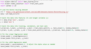
Evaluate Generalization Aspect of Linear, LASSO & Ridge Regression Models
Lets train the model once by splitting dataset into training, validation and test set to evaluate generalization aspect of the model. We can then select the final model. Here is the Python code:
from sklearn.linear_model import LinearRegression, Lasso, Ridge
from sklearn.metrics import mean_squared_error
from sklearn.model_selection import train_test_split
import pandas as pd

# Load the Boston Housing dataset
url = 'https://raw.githubusercontent.com/selva86/datasets/master/BostonHousing.csv'
data = pd.read_csv(url)

# Split the data into features (X) and target variable (y)
X = data.drop('medv', axis=1)
y = data['medv']

# Split the data into training, validation, and test sets
X_trainval, X_test, y_trainval, y_test = train_test_split(X, y, test_size=0.2, random_state=42)
X_train, X_val, y_train, y_val = train_test_split(X_trainval, y_trainval, test_size=0.25, random_state=42)

# Fit the Linear Regression model
linear_model = LinearRegression()
linear_model.fit(X_train, y_train)

# Fit the LASSO Regression model
lasso_model = Lasso(alpha=0.1)  # Adjust the alpha value as needed
lasso_model.fit(X_train, y_train)

# Fit the Ridge Regression model
ridge_model = Ridge(alpha=1.0)  # Adjust the alpha value as needed
ridge_model.fit(X_train, y_train)

# Evaluate the models using mean squared error (MSE) on validation and test sets
linear_val_mse = mean_squared_error(y_val, linear_model.predict(X_val))
lasso_val_mse = mean_squared_error(y_val, lasso_model.predict(X_val))
ridge_val_mse = mean_squared_error(y_val, ridge_model.predict(X_val))

linear_test_mse = mean_squared_error(y_test, linear_model.predict(X_test))
lasso_test_mse = mean_squared_error(y_test, lasso_model.predict(X_test))
ridge_test_mse = mean_squared_error(y_test, ridge_model.predict(X_test))

# Print the MSE values
print("Linear Regression:")
print("Validation MSE:", linear_val_mse)
print("Test MSE:", linear_test_mse)
print()

print("LASSO Regression:")
print("Validation MSE:", lasso_val_mse)
print("Test MSE:", lasso_test_mse)
print()

print("Ridge Regression:")
print("Validation MSE:", ridge_val_mse)
print("Test MSE:", ridge_test_mse)
Executing the above code will print the following:
Linear Regression:
Validation MSE: 22.3651
Test MSE: 25.298
LASSO Regression:
Validation MSE: 22.6615
Test MSE: 26.1317
Ridge Regression:
Validation MSE: 22.1929
Test MSE: 25.4528
Based on the MSE values, it can be seen that the Ridge Regression model performs slightly better than the Linear Regression model on the validation set, as it has the lowest validation MSE. However, on the test set, the Linear Regression model has a lower MSE compared to both LASSO and Ridge Regression models. This suggests that the Linear Regression model generalizes better to unseen data.
It’s important to note that the choice of the best model depends on the specific problem and the trade-off between bias and variance. In this case, although the Linear Regression model performs better on the test set, it is recommended to further evaluate the models using additional datasets (such as training and validation sets) to gain more insights into their performance and generalization ability. Cross-validation can also be employed to assess the models’ stability and select the most robust one.
Conclusion
Linear regression models can be built using Boston Housing Dataset to estimate house prices. While building models, we can use python code to preprocess the data, split it into training, validation, and test sets, and train the models. It is recommended to apply regularization techniques, namely LASSO and Ridge regression, to overcome potential issues such as overfitting and multicollinearity. By evaluating the models using metrics like Mean Squared Error (MSE), we can select the most appropriate model training using LinearRegression, Lasso, Ridge, LassoCV or RidgeCV. While the Linear Regression model showed promising results with lower MSE on the test set, further evaluation using additional datasets is recommended to assess their generalization aspect or we can also use cross validation (LassoCV, RidgeCV).
If you have any further questions, need clarification on any aspect discussed, or would like to explore similar topics in more detail, please don’t hesitate to reach out. I will be happy to help and provide further guidance.

Check out my latest book titled as First Principles Thinking: Building winning products using first principles thinking.
- Three Approaches to Creating AI Agents: Code Examples - June 27, 2025
- What is Embodied AI? Explained with Examples - May 11, 2025
- Retrieval Augmented Generation (RAG) & LLM: Examples - February 15, 2025
I found it very helpful. However the differences are not too understandable for me