Today when core businesses have started relying on machine learning (ML) models predictions, interpreting complex models has become a necessary requirement of AI governance (responsible AI). Data scientists are often asked to explain the inner workings of a machine learning models for understanding how the decisions are made. The Problem? Many of these models stand out as “black boxes“, delivering predictions without any comprehensible reasoning. This lack of transparency (especially in healthcare & finance use cases) can lead to mistrust in model predictions and inhibit the practical application of machine learning in fields that require a high degree of interpretability. It could lead to erroneous decision-making, or worse, legal and ethical complications. It also becomes a challenge for troubleshooting purpose.
But what if there was a way to demystify these models? What if you could easily understand and explain the predictions of your machine learning model, regardless of its complexity? Enter LIME, a powerful tool designed to help interpret the output of the “black box” models. In this blog post, we’ll explore how LIME (Local Interpretable Model-Agnostic Explanations) can be used to explain the features and predictions of a Linear Regression model using Python.
Before we get into the real action, lets have a quick overview on what’s LIME and how does it help with machine learning model?
What’s LIME & How does it help with Machine Learning Models?
LIME, which stands for “Local Interpretable Model-Agnostic Explanations,” is a popular tool in the realm of explainable artificial intelligence (AI). The primary goal of LIME is to provide human-understandable explanations for the predictions of any machine learning model. Here are some of the key features of LIME:
- Model-Agnostic: LIME is designed to work with any machine learning model. This includes simple linear models, decision trees, random forests, support vector machines, and even complex deep learning models.
- Local Fidelity: LIME explains the predictions of a model on a per-instance basis. It does this by approximating the model’s decision boundary only in the neighborhood of a particular instance.
- Interpretability: The main goal of LIME is to make the machine learning model’s predictions interpretable for humans. It achieves this by representing each explanation using a small number of interpretable features.
- Feature Selection: In order to ensure that the explanations are not too complex, LIME selects a small set of features that are most important for a particular prediction.
- Visualizations: LIME provides helpful visualizations that can give users an intuitive understanding of the model’s decision-making process.
LIME for Interpreting Machine Learning Model Predictions
In this section, we will look into how can we use LIME for interpreting the predictions of a Linear Regression machine learning model using the Boston Housing dataset. This dataset contains 13 features that influence the median value of owner-occupied homes. While Linear Regression models are intrinsically interpretable, for the sake of this example, we’ll assume a scenario where the model’s predictions require additional explanation.
Here is the Python code which demonstrates interpreting linear regression models output using LIME. Before executing the code, ensure you have installed LIME by using this command: !pip install lime
# Import necessary libraries
import pandas as pd
from sklearn.model_selection import train_test_split
from sklearn.linear_model import LinearRegression
from sklearn.metrics import mean_squared_error
from lime.lime_tabular import LimeTabularExplainer

# Load the dataset
url = 'https://raw.githubusercontent.com/selva86/datasets/master/BostonHousing.csv'
data = pd.read_csv(url)

# Split the data into features (X) and target (y)
X = data.drop('medv', axis=1)
y = data['medv']

# Split the data into training and test sets
X_train, X_test, y_train, y_test = train_test_split(X, y, test_size=0.2, random_state=42)

# Train a linear regression model
model = LinearRegression()
model.fit(X_train, y_train)

# Predict on the test set
y_pred = model.predict(X_test)

# Compute the mean squared error of the model
mse = mean_squared_error(y_test, y_pred)
print('Mean Squared Error:', mse)

# Initialize the explainer
explainer = LimeTabularExplainer(X_train.values, feature_names=X_train.columns, class_names=['medv'], verbose=True, mode='regression')

# Explain a prediction
i = 10  # index of the instance to be explained
exp = explainer.explain_instance(X_test.values[i], model.predict, num_features=5)

# Print the explanation
print('Instance:', i)
print('Prediction:', y_pred[i])
exp.show_in_notebook(show_table=True)
Note some of the following in the above code:
- The mean squared error (MSE) of the model is printed.
- The LIME explanation for the 10th instance in the test set is printed.
- The model interpretability is explained using the top 5 features that contributed to the prediction. However, the number of features should be used as per the requirements.
- An object of LimeTabularExplainer is initialized with the training data, feature names.
- The method explain_instance is invoked on the explainer object with a particular instance from our test set (10th instance) and the trained model’s predict function. The method returns an explanation object that contains information about which features were most influential for the prediction and how they contributed to it.
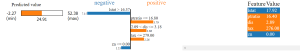
The following is the LIME output printed as part of executing of above code:

The following is the explanation of the above LIME output consisting of three different sections. It must be noted that LIME provides a local interpretation for specific predictions (such as 10th instance in current example). The interpretation includes both the direction (positive or negative) and magnitude (the weight) of the impact of the most important features.
- Predicted value section (left most): The “Predicted value” section shows the predicted median value of owner-occupied homes in $1000’s. The model’s prediction for the 10th instance taken up for analysis is 24.91. The minimum and maximum values of the prediction interval are -2.27 and 52.38 respectively.
- Negative & Positive section: This section shows the features that contribute to decreasing and increasing the predicted value respectively, along with their respective weights. Features with positive weights contribute to increasing the prediction value, while features with negative weights contribute to decreasing it. These features got determined by LIME to be the most influential for this specific prediction of this instance (10th instance).
- “lstat > 16.37” and “zn <= 0.00” are negatively affecting the predicted value. This suggests that a higher percentage of lower status of the population (lstat) and a lower proportion of residential land zoned for lots over 25,000 sq.ft. (zn) are associated with a lower median value of owner-occupied homes.
- “ptratio <= 16.80”, “2.09 < dis <= 3.18”, and “tax <= 279.00” are positively affecting the predicted value. This suggests that a lower pupil-teacher ratio by town (ptratio), weighted distances to five Boston employment centers (dis) within the specified range, and a full-value property-tax rate per $10,000 (tax) lower or equal to 279 are associated with a higher median value of owner-occupied homes.
- Feature Value section: The “Feature” and “Value” columns show the actual values of the top features for this instance (10th instance). For example, the percentage of lower status of the population (lstat) is 17.92, which is indeed greater than 16.37, thus negatively influencing the predicted value according to the model.
Conclusion
The importance of explainable AI in today’s data-driven landscape cannot be overstated. As data scientists, it’s of utmost importance to not only create machine learning models with high accuracy, but also to ensure their predictions are transparent, interpretable and understandable. With the help of LIME, the inner workings of these models can be understood and provide meaningful explanations for their predictions. LIME allows to understand the influence of individual features on specific predictions, offering a local, interpretable model of the original predictor. This local interpretation, although an approximation, provides valuable insights into the model’s decision-making process, enhancing our trust and confidence in its predictions.
Start by experimenting with LIME on your own datasets and models. Try it with different types of models – from decision trees and random forests to SVMs and neural networks. Recall that LIME is model-agnostic, making it a versatile tool in your machine learning toolkit. If you encounter any issues or have any questions while using LIME, don’t hesitate to reach out.

Check out my latest book titled as First Principles Thinking: Building winning products using first principles thinking.
- Mathematics Topics for Machine Learning Beginners - July 6, 2025
- Questions to Ask When Thinking Like a Product Leader - July 3, 2025
- Three Approaches to Creating AI Agents: Code Examples - June 27, 2025
I found it very helpful. However the differences are not too understandable for me