Types of Probability Distributions: Codes, Examples

In this post, you will learn the definition of 25 different types of probability distributions. Probability distributions play an important role in statistics and in many other fields, such as economics, engineering, and finance. They are used to model all sorts of real-world phenomena, from the weather to stock market prices. Before we get into understanding different types of probability distributions, let’s understand some fundamentals. If you are a data scientist, you would like to go through these distributions. This page could also be seen as a cheat sheet for probability distributions.

What are Probability Distributions?

Probability distributions are a way of describing how likely it is for a random variable to take on different possible values. In other words, they provide a way of quantifying the chances of something happening. For example, lets take a random variable X as number of times “heads” occur when a coin is flipped 5 times. X can take values such as 1, 2, 3, 4 and 5. Lets say X = 2. That would mean that head will occur for 2 times. Probability distribution for X would mean what is the probability that X can take values of 1, 2, 3, 4 and 5. It can be denoted as P(X=1), P(X=2), P(X=3), P(X=4), P(X=5). There are many different types of distributions described later in this post, each with its own properties. Some of the most common examples include the uniform distribution, the normal distribution, and the Poisson distribution.

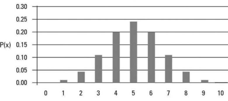
Probability distributions are often graphed as histograms, with the possibilities on the x-axis and the probabilities on the y-axis. In the above example, the X axis will consist of values such as 1, 2, 3, 4 and 5. And the Y-axis will consist of values such as P(X=1), P(X=2), P(X=3), P(X=4), P(X=5). The picture below represents the probability distribution of random variable X taking value 1 to 10.

Probability distributions are divided into two classes:

• Discrete Probability Distribution: Discrete probability distribution is a mathematical function that calculates the probabilities of outcomes of discrete random variables. In other words, it helps to determine the likelihood that a random variable will take on a given value within well-defined range. For example, probability of number of heads occurring in 10 coin flips can be termed as discrete probability distribution. The example shown above is an example of discrete probability distribution. A discrete probability distribution assigns a probability to each discrete outcome of a random variable. Discrete probability distributions are often used to model events that can only have certain outcomes, such as the roll of a die or the flip of a coin. However, they can also be used to model more complex phenomena, such as the number of visitors to a website on a given day. Discrete probability distributions are generally classified according to the type of random variable they express. The most common type of discrete probability distribution is the Binomial distribution, which is used to model events with two possible outcomes, such as success and failure. Some additional examples of the discrete probability distribution include the Bernoulli’s distribution, the geometric distribution, and the negative binomial distribution. The discrete probability distribution can be represented using a probability mass function (PMF).
• Continuous Probability Distribution: A continuous probability distribution is a type of probability distribution that deals with random variables that can take on any continuous value within a certain range. Continuous random variables are opposed to discrete random variables, which can only take on specific, discrete values. Common examples of continuous random variables include things like height, weight, and volume. Continuous probability distributions are often used to model physical phenomena, such as the rate of radioactive decay or the speed of sound waves. There are several different types of continuous probability distributions, each with its own shape. The most common is the Normal distribution, which is bell-shaped. Many real-world phenomena can be described using continuous probability distributions. For example, the height of students in a classroom might be described by a continuous probability distribution. The distribution would take into account the fact that some students are taller than others, but it would also allow for the possibility of any height being observed. Similarly, the weight of newborn babies might also be described by a continuous probability distribution. This would allow for the fact that some babies are born heavier than others, but it would also allow for the possibility of any weight being observed. In both cases, the continuous nature of the distribution reflects the continuous nature of the underlying phenomenon.

Different Types of Probability Distributions

Here is the list of different types of probability distributions:

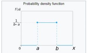
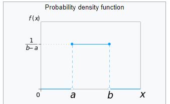
1. Uniform distribution: Also known as rectangular distribution, the uniform distribution is a type of probability distribution that has a constant probability. Simply speaking, a uniform probability distribution represents the probability distribution in which all outcomes have the equal probability. The uniform probability distribution is often used in situations where there is no clear “favorite” outcome and all outcomes are equally likely. For example, when flipping a coin, the two possible outcomes (heads or tails) are both equally likely, so a uniform probability distribution can be used to model the flip. Similarly, when rolling a die, all six outcomes are equally likely, so a uniform probability distribution can again be used. The uniform probability distribution is a very important tool in statistics and is used in many real-world applications.
   
   
   
   Here is the Python code for working with the uniform probability distribution: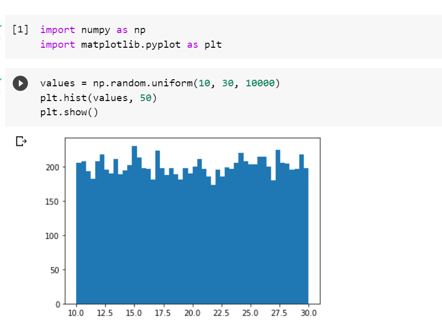
   
   
   
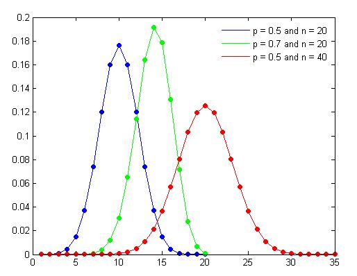
2. Binomial distribution: Binomial probability distribution is a probability distribution that gives the likelihood of a given number of successful outcomes in a fixed number of trials. It is a discrete probability distribution that is used to model the number of successes in a sequence of n independent trials or a fixed number of Bernoulli trials, each asking a yes-no question. Each experiment has boolean-valued outcome such as success/yes/true/one (with probability p) or failure/no/false/zero (with probability, q = 1 − p).  The distribution is then calculated by taking the product of n and p and then raised to the power of n. This results in a bell-shaped curve, with the mean equal to np and the standard deviation equal to √np(1-p). The following conditions need to be satisfied for the experiment to be termed as a binomial experiment: A. Fixed number of n trials. B. Each trial is independent. C. Only two outcomes are possible (Success and Failure). D. The probability of success (p) for each trial is constant. E. A random variable Y= the number of successes. This type of probability calculation is important in many fields, from insurance and finance to manufacturing and quality control. In each case, understanding the binomial probability distribution can help decision-makers make better choices and plan for different outcomes.
   Here are some examples of binomial distribution:
   • For a coin tossed N times, binomial distribution can be used to model the probability of the number of successes (say, heads). For example, for the coin toss 10 times, the binomial distribution could be used to model the probability of a number of heads (1 to 10).
   • Here is the sample binomial distribution plot created with different values of n and p
     
     
     
3. Multinomial distribution: It allows us to calculate the probability of observing a given combination of outcomes from n trials, where each trial can have more than two possible outcomes. The Multinomial Distribution is often used in situations where there are more than two mutually exclusive outcomes, and we are interested in the probability of observing a given combination of those outcomes. In the real world, there are many examples of multinomial probability distributions. For example, consider flipping a coin three times. There are eight possible outcomes: {HHH, HHT, HTH, HTT, THH, THT, TTH, TTT}. The probability of each outcome can be calculated using the Multinomial Probability Formula. In this formula, “n” represents the number of trials (in this case, three), and “p1”, “p2”, and “p3” represent the probabilities of each outcome (in this case, 1/8 for each outcome).
   
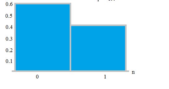
4. Bernoulli distribution: A discrete or categorical probability distribution for a Bernoulli trial. For n = 1 (one experiment), binomial distribution can be termed as Bernoulli distribution. The Bernoulli distribution is often termed as a special case of the binomial distribution, where n = 1.  A single success/failure experiment is also called a Bernoulli trial or Bernoulli experiment and a sequence of outcomes is called a Bernoulli process. The following is a Bernoulli distribution. In the plot given below, the probability of the failure is labeled on the x-axis as 0 and success is labeled as 1. The probability of success (1) is 0.4, and the probability of failure (0) is 0.6. Here is a great read on Bernoulli distribution.
   
   
   
5. Negative Binomial distribution: A discrete probability distribution of the number of trials in a sequence of independent and identically distributed Bernoulli trials before a specified or fixed number of successes occurs. Sometimes, the negative binomial distribution has also defined as a probability distribution of number of successes needed to get a fixed number of failures or vice-versa. The negative binomial experiment is almost the same as a binomial experiment with one difference: a binomial experiment has a fixed number of trials. The negative binomial distribution is known as the Pascal distribution. Here are some examples/scenarios which can be modeled using negative binomial distribution:
   • In case of tossing a coin, the negative binomial distribution can give the number of trials required to happen before a certain number of heads appear
   • The negative binomial distribution can be used to model the number of the goal attempts an athlete makes before scoring r goals, though. 
   • The negative binomial distribution can be used to model the number of days a certain machine works before it breaks down.
   • Take a standard deck of cards, shuffle them, and choose a card. Replace the card and repeat until you have drawn two aces. Y is the number of draws needed to draw two aces. As the number of trials isn’t fixed (i.e. you stop when you draw the second ace), this makes it a negative binomial distribution.
     
     Here is a sample plot representing negative binomial distribution: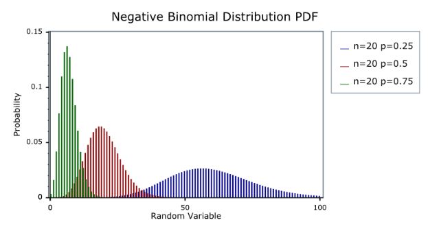
     
     
     
     
6. Normal distribution: A type of continuous probability distribution for a real-valued random variable. It is a type of symmetric distribution where most of the observations cluster around the central peak and the probabilities for values further away from the mean taper off equally in both directions. It is represented using a bell-shaped density curve described by its mean and standard deviation. It is also known as the Gaussian distribution. It has got the following features:
   • Symmetric bell shape
   • Mean and median are equal; both located at the center of the distribution
   • 68% of the data falls within 1 standard deviation of the mean
   • 95% of the data falls within 2 standard deviations of the mean
   • 99.7% percent of the data falls within 3 standard deviations of the mean
     
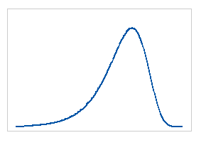
     Here is a sample normal distribution curve: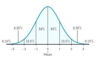
     
     
     
     Here is the Python code for normal distribution. norm class of scipy.stats module is used to calculate probability of input ranging from -3 to 3 with an interval of 0.001 using norm.pdf probability density function. The plot represents normal distribution.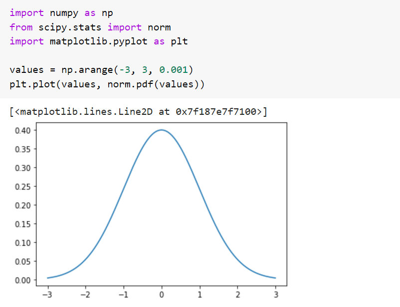
     
     
     
     
7. Poisson distribution: A Poisson distribution is a discrete probability distribution that shows how many times an event is likely to occur within a fixed interval of time or space if these events occur with a known average rate and independently of the time since the last event. It is used for independent events that occur at a constant rate within a given interval of time. Note that Poisson distribution is associated with both time and space. Another key point is that events need to be independent of each other. When to use Poisson distribution? Poisson distribution is used for finding the probability of a number of events in a time period or finding the probability of waiting some time until the next event. Here is a great read on Poisson distribution. Here are some examples:
   • Customers calling a help center: On average, there are, say, 10 customers which call in an hour. Thus, Poisson distribution can be used to model the probability of a different number of customers calling within an hour (say, 5 or 6 or 7 or 8 or 9 or 11 customers, etc). The diagram below represents
   • No. of visitors to a website: On average, there are 500 visitors to a website every day. Poisson distribution can be used to estimate the number of visitors every day.
   • Radioactive decay in atoms
   • Photons arriving at a space telescope
   • Movements in a stock price
   • Number of trees in a given acre of land
     
     Here is a sample diagram representing the probability distribution for a given lambda (rate of change of event)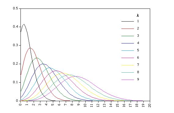
     
     
     
8. Lognormal distribution: A continuous distribution in which the logarithm of a variable has a normal distribution. In other words, Lognormal distribution is a probability distribution with a normally distributed logarithm. A random variable is log-normally distributed if its logarithm is normally distributed. Skewed distributions with low mean values, large variance, and all-positive values often fit this type of distribution. Some of the other names of the Lognormal distribution are Galton, Galton-McAlister, Gibrat, Cobb-Douglas distributions. Here are some examples of the lognormal distributions:
   • Size of silver particles in a photographic emulsion
   • Survival time of bacteria in disinfectants
   • The weight and blood pressure of humans
   • The number of words written in sentences by George Bernard Shaw
   • Milk production by cows.
   • Lives of industrial units with failure modes that are characterized by fatigue-stress.
   • Amounts of rainfall.
   • Size distributions of rainfall droplets.
   • The volume of gas in a petroleum reserve.
     
9. 3-parameter Lognormal distribution: The 3-parameter lognormal distribution is a general skew distribution in which the logarithm of any linear function of a given variable is normally distributed. The three-parameter lognormal distribution is frequently used in the hydrologic analysis of extreme floods, seasonal flow volumes, duration curves for daily streamflow, rainfall intensity-duration, soil water retention.
   
10. Exponential distribution: Exponential distribution is a continuous probability distribution that describes the waiting time until the next event (success, failure, arrival, etc) in a Poisson process. Taking the cue from the example sighted in the Poisson distribution in this post, the probability distribution used to model the time between every customer calls is the exponential distribution. Recall that the Poisson distribution is used to model the probability distribution of the number of customer calls within an hour given a particular rate (lambda). Simply speaking, the exponential distribution could be used to model the waiting time before the next event occurs. This is one of the commonly used distributions in reliability engineering. Here are some examples of exponential distribution:
    • How much time will go before a customer call happens?
    • How much time will go before the next customer arrive in the shop?
    • How much time will pass by before the next robbery happens in any part of the city?
    • How much time will pass by before the next childbirth in the city?
    • How much time will go until the customer finishes browsing and actually purchases something in your store (success)?
    • How much time will go until the hardware on AWS EC2 fails (failure)?
    • How much time will go until the bus arrives (arrival)?
      
      Here is the sample plot representing the exponential distribution: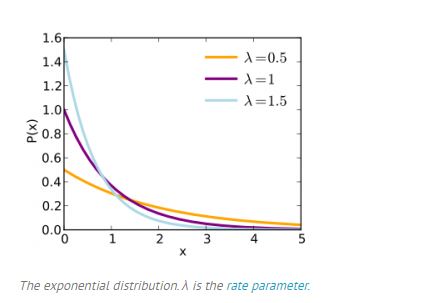
      
      
      
      Here is the sample Python code which can be used to create plot for exponential distribution: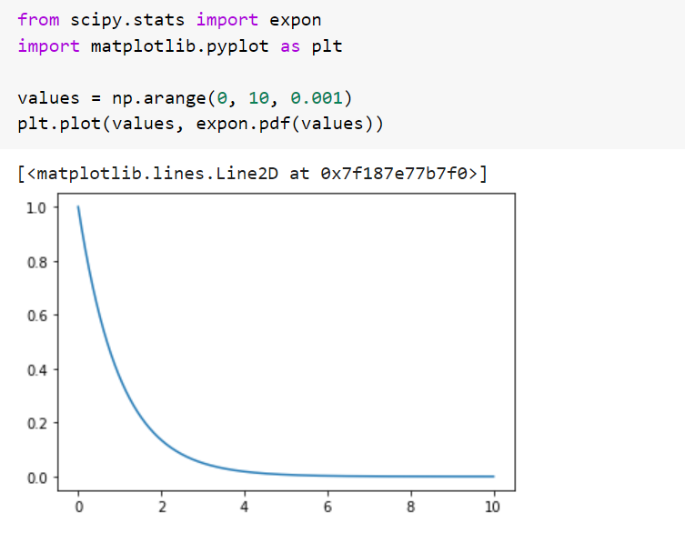
      
      
      
11. 2-parameter Exponential distribution
12. Weibull distribution: A type of continuous probability distribution, the Weibull distribution has the ability to assume the characteristics of many different types of distributions. It is flexible enough to model a variety of data sets, be it right-skewed, left-skewed or symmetrical dataset. Generally speaking, the Weibull distribution is determined by 2-parameters such as shape and scale. The location parameter is set to zero. Here are some of the examples where Weibull distribution is used for modeling the related random variable.
    • Reliability engineering, life data, and failure analysis
    • In electrical engineering to represent overvoltage occurring in an electrical system
    • In survival analysis
    • In weather forecasting and the wind power industry to describe wind speed distributions, as the natural distribution often matches the Weibull shape
    • In information retrieval to model dwell times on web pages
    • In general insurance to model the size of reinsurance claims, and the cumulative development of asbestosis losses
    • In hydrology, extreme events such as annual maximum one-day rainfalls and river discharges
      
      Here is a sample plot representing Weibull distribution for different value of shape parameter: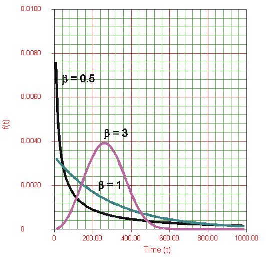
      
      
      
13. 3-parameter Weibull distribution: In 3-parameter Weibull distribution, apart from shape and scale, the location parameter also becomes important.
    
14. Dirichlet distribution: A type of continuous probability distribution. The Dirichlet distribution is a probability distribution over the space of multinomial distributions. It is the probability distribution over a probability simplex – a bunch of numbers that add up to 1. The following is an example of probability simplex:
    
    (0.7, 0.3)
    (0.2, 0.1, 0.7)
    (0.07, 0.2, 0.13, 0.1, 0.2, 0.3)
    
    The above numbers represent probabilities over K distinct categories. In the above examples, K is 2, 3, and 6 respectively. That’s why they are also called categorical distributions
    
    Dirichlet distributions are commonly used as the prior distributions in Bayesian statistics. It is a multivariate generalization of the beta distribution. Thus, it is also termed a multivariate beta distribution.
    
15. Beta distribution: A type of continuous probability distribution, Beta distribution is defined on the interval [0, 1] parameterized by two positive shape parameters α and β, that appear as exponents of the random variable and control the shape of the distribution. Simply speaking, Beta distribution is used to represent percentages, proportion or probability outcomes. It can also be said as the distribution of probabilities. Here are some examples which could be modeled using beta distribution:
    • How likely it is that the preferred candidate for mayor will receive 70% of the vote. 70% of the vote (0.7) here is the proportion or probability that falls in the limit [0,1].
    • How likely is that President Trump will win 2020 presidential elections? Note the value will fall within the limit [0, 1]
      
      Check out this post sighting example of how beta distribution could be used to model the probability of runs that could be scored in upcoming cricket match.
      
16. Gamma distribution: Gamma distribution is a continuous probability distribution that is used to model the continuous variables that are always positive and have skewed distributions. It is a two-parameter family of continuous probability distributions. The exponential distribution, Erlang distribution, and chi-squared distribution are special cases of the gamma distribution.  It is a distribution that arises naturally in processes for which the waiting times between events are relevant. It can be thought of as a waiting time between Poisson distributed events. Here are some of the examples of a gamma distribution:
    • In life testing, the waiting time until death is a random variable that is frequently modeled with a gamma distribution
    • The size of loan defaults or aggregate insurance claims
    • The flow of items through manufacturing and distribution processes
    • The load on web servers
    • The many and varied forms of telecom exchange
      
17. 3-parameter Gamma distribution: Also called as a generalized gamma distribution, 3-parameter Gamma distribution is a type of continuous probability distribution with three parameters. Since many distributions commonly used for parametric models in survival analysis (such as the Exponential distribution, the Weibull distribution, and the Gamma distribution) are special cases of the generalized gamma, it is sometimes used to determine which parametric model is appropriate for a given set of data.
    
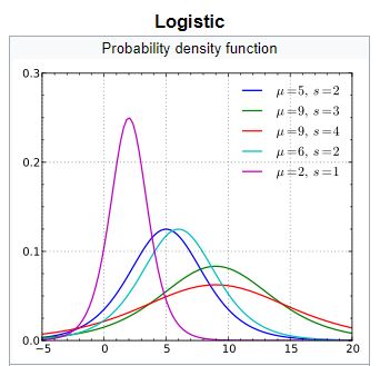
18. Logistic distribution: A continuous probability distribution, whose cumulative distribution function is the logistic function, which appears in logistic regression and feedforward neural networks. It resembles the normal distribution in shape but has heavier tails (higher kurtosis). Here is the sample plot representing the logistic distribution for different location and shape parameter:
    
    
    
19. Turkey Lambda distribution: A continuous, symmetric probability distribution defined in terms of its quantile function, and is typically used to identify an appropriate distribution. The Tukey lambda distribution is symmetric around zero, therefore the expected value of this distribution is equal to zero. The most common use of this distribution is to generate a Tukey lambda PPCC plot of a data set. Based on the PPCC plot, an appropriate model for the data is suggested.
    
20. Log-Logistic distribution: The probability distribution of a random variable whose logarithm has a logistic distribution. It is similar in shape to the log-normal distribution but has heavier tails. Here are some examples of scenarios that are modeled using Log-logistic distribution:
    • Used in survival analysis as a parametric model for events whose rate increases initially and decreases later, as, for example, the mortality rate from cancer following diagnosis or treatment.
    • Used in hydrology to model streamflow and precipitation,
    • Used in economics as a simple model of the distribution of wealth or income
    • Used in networking to model the transmission times of data considering both the network and the software.
      
      Here is a sample plot representing Log-Logistic distribution: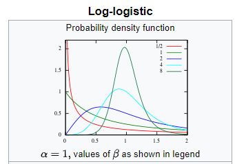
      
      
      
21. 3-parameter Log-Logistic distribution: 3-parameter log-logistic distribution is a generalization of the two–parameter log–logistic distribution.  It has been applied to the frequency analysis of precipitation and streamflow data.
    
22. Smallest extreme value distribution: This distribution is used to model time to failure for a system that fails when its weakest component fails. It is defined by its location and scale parameters. Skewed to the left, the smallest extreme value distribution describes extreme phenomena such as the minimum temperature and rainfall during a drought.  Here is the sample plot representing the smallest extreme value distribution
    
    
    
23. Largest extreme value distribution: The largest extreme value distribution is used to model the maximum value from a distribution of random observations. Skewed to the right, it describes extreme phenomena such as extreme wind velocities and high insurance losses. For example, the distribution of the water levels in river overtime is frequently skewed to the right with a few cases of extreme water levels to the right and a majority of water levels in the lower tail. Here is the sample plot representing the largest extreme value distribution:
    
    
    
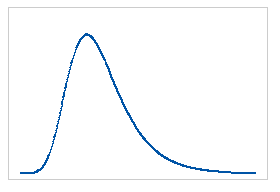
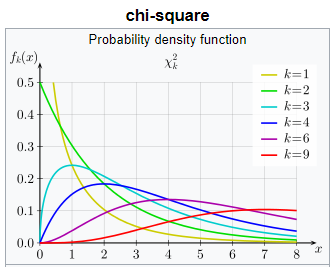
24. Chi-square distribution: Chi-squared distribution with k degrees of freedom is the distribution of a sum of the squares of k independent standard normal random variables. It is a special case of the gamma distribution and is one of the most widely used probability distributions in inferential statistics, notably in hypothesis testing and in construction of confidence intervals. It is used in the common chi-square tests for some of the following reasons:
    • The goodness of fit of an observed distribution to a theoretical one
    • The independence of two criteria of classification of qualitative data
    • In confidence interval estimation for a population standard deviation of a normal distribution from a sample standard deviation. 
      
      Here is a sample chi-square distribution plot:
      
      
      
25. Geometric distribution: The geometric distribution is the probability distribution of the number of trials needed to get the first success in repeated independent Bernoulli trials. In other words, the Geometric distribution can also be defined as a number of failures before the first success happens or vice-versa. The geometric distribution is an appropriate model if the following assumptions are true.
    • The phenomenon being modeled is a sequence of independent trials.
    • There are only two possible outcomes for each trial, often designated success or failure.
    • The probability of success, p, is the same for every trial.

There are many more probability distributions such as some of the following which I will be covering in the following posts.

• Tweedie
• Wishart
• Inverse Gamma
• Laplace
• Log-Laplace
• Cauchy
• Inverse Chi-squared

References

• Why Weibull distribution is always welcome
• Characteristics of Weibull distribution
• Understanding beta distribution (using baseball statistics)
• What is the beta distributions?
• Visualizing Dirichlet distributions with Matplotlib
• Dirichlet distributions
• Dirichlet distribution: Simple definition, PDF, Mean
• Quora – Intuitive explanation of Dirichlet distribution
• Smallest and largest extreme value distribution
• Logistic distribution
• Log-logistic distribution
• Exponential distribution – Intuition, applications
• Intuition behind beta distribution

• Author
• Recent Posts

Follow me

Ajitesh Kumar

I have been recently working in the area of Data analytics including Data Science and Machine Learning / Deep Learning. I am also passionate about different technologies including programming languages such as Java/JEE, Javascript, Python, R, Julia, etc, and technologies such as Blockchain, mobile computing, cloud-native technologies, application security, cloud computing platforms, big data, etc. For latest updates and blogs, follow us on Twitter. I would love to connect with you on Linkedin.
Check out my latest book titled as First Principles Thinking: Building winning products using first principles thinking. Check out my other blog, Revive-n-Thrive.com

Follow me

Latest posts by Ajitesh Kumar (see all)

• Mean Squared Error vs Cross Entropy Loss Function - April 28, 2024
• Cross Entropy Loss Explained with Python Examples - April 28, 2024
• Logistic Regression in Machine Learning: Python Example - April 26, 2024