Random variables are one of the most important concepts in statistics. In this blog post, we will discuss what they are, their different types, and how they are related to the probability distribution. We will also provide examples so that you can better understand this concept. As a data scientist, it is of utmost importance that you have a strong understanding of random variables and how to work with them.
What is a random variable and what are some examples?
A random variable is a variable that can take on random values. The key difference between a variable and a random variable is that the value of the random variable cannot be predicted with certainty. Random variables can be both scaler and vector-valued. A vector-valued random variable can take on different sets of values at a different point in time. Some examples of random variables include:
- X: No. of times 6 occurs in the dice rolled for 10 times: X can take value of 1 to 10 with 1 and 10 having least probability.
- X: No. of heads occurring the coin flipped for 10 times: X can take value of 1 to 10 with 1 and 10 having least probability.
- X: Number of students scoring more than 80 marks in a test
- X: The number of people coming to the shop between 11 AM and 12:00 PM: X can take value from 1 to N with varying probabilities.
- X: Number of cars passing a building between 9 and 10 AM
- X: Number of people traveling by flight on any particular day from an airport
- X: Number of sales on any particular day
- X: Number of people visiting a website on any particular day
Random variables are denoted using uppercase letters. For example, X can be used to denote a random variable. If we have two random variables, say X and Y, then we can use the notation (X, Y) to represent them.
P(X = x) represents the probability of the random variable X taking on a particular value, x. For example, When X represents no. of heads in coin flipped for 10 times, P(X=5) represents the probability that the number of heads takes the value of 5. In other words, X = 5.
How are random variables related to the probability distribution?
As mentioned above, the random variables are variables whose values can’t be predicted with certainty. Thus, the random variables must be associated with the probability distribution which specifies the probability of the random variable taking different values. For example, when X represents the count that dice occurs as 6 when rolled for 8 times, probability distribution of this random variable will include values of P(X=1), P(X=2), P(X=3), P(X=4), P(X=5), P(X=6), P(X=7), P(X=8)
The probability distribution of a random variable is a function that maps values that the random variable can take to their corresponding probabilities. In other words, it tells us how likely it is for the random variable to take on each value. The most common type of probability distribution is the normal distribution or Gaussian distribution. Other types include uniform distributions, binomial distributions, and Poisson distributions.
Types of random variables & probability distributions
Random variables can be of two different types:
- Discrete random variables
- Continuous random variables
Discrete random variables: These types of random variables can take on only a countable number of values be it a small or large number. Some examples of discrete random variables are:
- The number of students in a classroom
- The number of cars sold by a company in a day
- The number of people visiting a website in an hour
The probability distribution of discrete random variables can be calculated using what is called the probability mass function (PMF). PMF is a function that assigns probabilities to discrete outcomes. Probability mass functions can be applied to many discrete random variables at the same time to determine the probability distribution which is called a joint probability distribution. P(X=x, Y=y) denotes the probability that X is equal to x and Y is equal to y simultaneously.
Continuous random variables: These types of random variables can take on any real value. Some examples of continuous random variables are:
- The time taken to complete a task
- The height of a person
- The weight of a person
- The income of a person
The probability distribution of a continuous random variable can be calculated using what is called the probability density function (PDF). PDF is a function that assigns probabilities to continuous outcomes. The probability of a continuous random variable taking on any particular value is 0 but the probability of it taking values in a range is non-zero. To calculate the probability, we need to integrate the PDF over that range.
How to work with random variables in Python
In Python, the random variable having integer values can be generated using the randint() function in the random module. This function takes two parameters: the lower limit & upper limit.
For example, if we want to generate a random variable that can take on integer values between 0 and 100, we will use the following code:
import numpy as np
X = np.random.randint(0, 100)
print(X)
We can also generate an array of floats using the rand() function in the NumPy library. The rand() function takes a shape parameter that specifies the size of the array. For example, if we want to generate an array of floats with shape (10, ), we will use the following code:
import numpy as np
X = np.random.rand(10)
X
To calculate the probability distribution of a discrete random variable, we can use the scipy.stats library in Python. The scipy.stats library contains a number of probability distributions as well as functions to calculate different statistical properties such as mean, variance, etc.
For example, let’s say we have a random variable X that can take five different values having different probabilities. We can calculate the probability distribution using the following code:
'''
Print the discrete random variable
'''
from scipy.stats import rv_discrete
import numpy as np

x = np.arange(5)
P_x = [0.1, 0.4, 0.3, 0.1, 0.1]
X = rv_discrete(name='X', values=(x, P_x))
print(X.pmf(x))
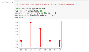
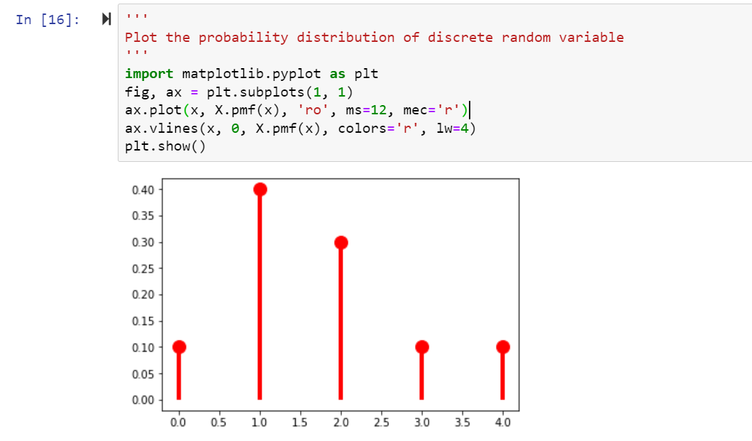
The above probability distribution can be plotted using the following code:
'''
Plot the probability distribution of discrete random variable
'''
import matplotlib.pyplot as plt
fig, ax = plt.subplots(1, 1)
ax.plot(x, X.pmf(x), 'ro', ms=12, mec='r')
ax.vlines(x, 0, X.pmf(x), colors='r', lw=4)
plt.show()
The following is how the probability distribution plot will be created based on the above code:
Conclusion
In conclusion, random variables are an important concept in statistics that allows us to model events that have uncertainty. There are two main types of random variables: discrete and continuous. Discrete random variables can take on only a countable number of values while continuous random variables can take on any real value. The probability distribution of a random variable specifies the probabilities of the possible outcomes representing different values of the random variable. For the discrete random variables, the function mapping the probability value to individual outcomes is called probability mass function (PMF). For the continuous random variables, the function mapping the probability value to individual outcomes is called probability density function (PDF).

Check out my latest book titled as First Principles Thinking: Building winning products using first principles thinking.
- Mathematics Topics for Machine Learning Beginners - July 6, 2025
- Questions to Ask When Thinking Like a Product Leader - July 3, 2025
- Three Approaches to Creating AI Agents: Code Examples - June 27, 2025
I found it very helpful. However the differences are not too understandable for me