
Last updated: 16th Nov, 2023
Histograms are a graphical representation of the distribution of data. In Python, there are several ways to create histograms. One popular method is to use the Matplotlib library. In this tutorial, we will cover the basics of Histogram Plots and how to create different types of Histogram plots using the popular Python libraries, Matplotlib and Pandas. We will also explore some real-world examples to demonstrate the usefulness of Histogram Plots in various industries and applications. As data scientists, it is important to learn how to create visualizations to communicate our findings. Histograms are one way to do this effectively.
What are Histogram plots?
Histogram plots are a way of representing the distribution of data. It is an estimate of the probability distribution of a continuous or discrete variable. To construct a histogram, the first step is to “bin” the range of values—that is, divide the entire range of values into a series of intervals—and then count how many values fall into each interval. The bins are usually specified as consecutive, non-overlapping intervals of a variable. The Histogram Plot displays these bins as adjacent bars, with the height of each bar representing the frequency (or count) of data points within that bin.
The following represents key components of a Histogram:
-
Bins: These are the intervals into which the data range is divided. The choice of the number of bins and their width can greatly affect the appearance of the histogram, and thus the interpretation of the data. Generally, more bins lead to a more detailed view of the data distribution, while fewer bins provide a more generalized view.
- Range: The range of a Histogram Plot is the span of values covered by the bins. It can be defined by the user or automatically calculated based on the data.
-
Frequency: The frequency is the number of data points that fall into each bin. In a Histogram Plot, the height of each bar represents the frequency of the corresponding bin.
-
Density: In some cases, it’s useful to normalize the histogram by the total number of data points. This creates a probability density, which allows you to compare histograms with different sample sizes or bin widths.
Let’s understand the concept of Histogram plots with the help of an example. Let’s say we want to understand how age of all the passengers is distributed on any particular day within an airport. On a particular 1500 passengers visited the airport (hypothetically). Let’s say hypothetically speaking, the goal is to use this data to determine how do I see advertisement space at different places in the airport. So, this is how the histogram would look like:

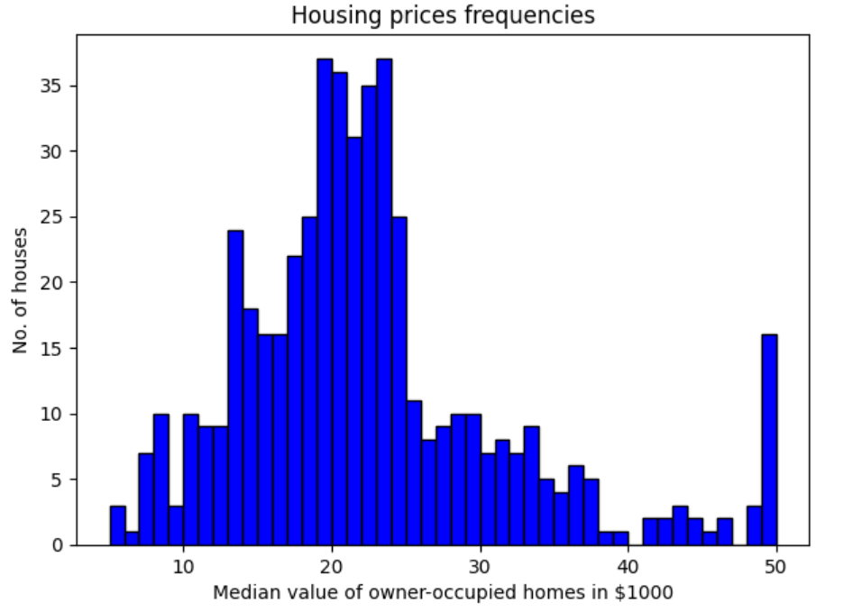
Note that histograms are generated by binning the data. Their visual appearance would depend on the choice of the bin width. Thus, it is imperative that one should select most appropriate bin width rather than relying on default bind width chosen by the visualization program. If the bin width set is too small, then the histogram becomes overly peaky and visually busy as like the above diagram where the bin width is set to 5. If the bin width is too large, then smaller features in the distribution of the data may disappear.
Difference: Are Histograms and Bar Plots one and the same thing?
One confuses histograms with bar plots which are used to represent the categorical data. Histograms are used to represent the data distribution of continuous or discrete data while bar plots or bar charts are used to represent comparisons between categorical data. Here are few differences you would want to keep in mind:
- Purpose: Histograms are primarily used to analyze the distribution, skewness, and modality of a dataset, as well as to discover patterns, trends, and potential outliers. Bar charts, on the other hand, are used to compare different categories or groups, highlighting differences or similarities between them.
- Types of data: In a histogram, the data is divided into a set of intervals (bins), and the height of each bar represents the frequency of data points within that interval. In a bar chart, each bar represents a distinct category, and the height of each bar indicates the value or count associated with that category.
- Spacing between bars: In a histogram, the bars are usually adjacent, without any gaps, because the data is continuous or discrete but ordered. This represents the continuous nature of the underlying data. In a bar chart, there is usually spacing between the bars, emphasizing that each bar represents a separate, unrelated category.
- Axes: In a histogram, both the x and y axes represent numerical values. The x-axis represents the bins or intervals into which the data range is divided, and the y-axis represents the frequency (count) of data points within each bin. In a bar chart, the x-axis represents distinct categories, while the y-axis represents numerical values or counts associated with each category.
Most Common Issues while Creating Histogram Plots
Creating histogram plots can sometimes pose challenges, especially for those new to data visualization or working with complex datasets. Here are some of the most common issues encountered:
- Inappropriate Bin Size: Choosing the right number of bins or bin width is crucial. Too many bins can make the data appear noisy, while too few can oversimplify the distribution, hiding important details.
- Data Range and Outliers: Outliers or a wide range of data can skew the histogram, making it difficult to interpret the main distribution of the data.
- Lack of Visual Clarity: Issues with visual clarity, such as poor choice of colors, lack of labels, or overlapping labels, can make the histogram hard to read and understand.
- Non-Numerical Data: Histograms are meant for numerical data. Attempting to create a histogram with non-numerical (categorical) data can lead to errors or misleading representations.
- Incorrect Data Binning: Misunderstandings about how data are binned (e.g., inclusive vs. exclusive bin edges) can lead to incorrect interpretations.
- Handling Missing Values: Not properly handling missing or NaN values can distort the histogram or cause errors during plotting.
- Comparing Different Distributions: Creating histograms that effectively compare different distributions (e.g., overlaying histograms) requires careful attention to scale, color, and transparency.
- Software-specific Issues: Depending on the software or library (like Pandas, Matplotlib, or Seaborn in Python), users may encounter syntax errors, compatibility issues, or limitations in customization options.
- Understanding Statistical Significance: Interpreting histograms in the context of statistical significance and understanding what patterns are meaningful can be challenging, especially for those less experienced in statistical analysis.
Plotting Histogram using Matplotlib & Pandas
There are a few things to keep in mind when creating histograms using Matplotlib and Pandas package:
- We can create a histogram from a Pandas DataFrame using the Matplotlib plot() function.
- We can specify the number of bins using the bins parameter.
- We can specify the range of values to include in the histogram using the range parameter.
- We can make our histogram look nicer by using colors and adding title and labels.
To create a Histogram plot using the Matplotlib and Pandas library, you first need to import the Matplotlib.pyplot and Pandas.
import matplotlib.pyplot as plt
import pandas as pd
Once the module is imported, you can create a Histogram object by passing in the data that you want to plot. The data can be passed as one column of data frame or the list of data depending upon the type of Histogram you want to plot. In this section you will learn how to create a histogram plot on a dataframe column, multiple histogram plots representing data related to different class of data and stacked histogram. The boston housing prices dataset is used for plotting Histogram in this section.
Plotting Histogram using Matplotlib on one column of a Pandas DataFrame
To plot a Histogram using Matplotlib, you need to first import the Histogram class from the Matplotlib library. The Histogram class has a plot() method which is used to plot histograms. The plot() method accepts a dataframe column as an argument. The Histogram will be plotted on the column of the dataframe.
In the code below Boston housing price sklearn.datasets has been imported and a Pandas dataframe is created. Thereafter, a histogram is plotted using Matplotlib on the target column ‘MEDV’.
import pandas as pd
import numpy as np
from sklearn import datasets
import matplotlib.pyplot as plt
import matplotlib
%matplotlib inline
matplotlib.rcParams['font.size'] = 10
matplotlib.rcParams['figure.dpi'] = 100
from IPython.core.pylabtools import figsize
# Load boston housing price dataset
housing_prices = datasets.load_boston()
# Create Pandas dataframe
hp_data_transpose = housing_prices.data.transpose()
df_hp = pd.DataFrame({
  'CRIM': hp_data_transpose[0],
  'ZN':hp_data_transpose[1],
  'INDUS':hp_data_transpose[2],
  'CHAS':hp_data_transpose[3],
  'NOX':hp_data_transpose[4],
  'RM':hp_data_transpose[5],
  'AGE':hp_data_transpose[6],
  'DIS':hp_data_transpose[7],
  'RAD':hp_data_transpose[8],
  'TAX':hp_data_transpose[9],
  'PTRATIO':hp_data_transpose[10],
  'B':hp_data_transpose[11],
  'LSTAT':hp_data_transpose[12]
})
df_hp['MEDV'] = housing_prices.target
# Create histogram on MEDV column (target column)
figsize(7, 5)
plt.hist(df_hp['MEDV'], color='blue', edgecolor='black', bins=int(45/1))
plt.xlabel('Median value of owner-occupied homes in $1000')
plt.ylabel('No. of houses')
plt.title('Housing prices frequencies')
Executing the above code will print the following Histogram.
Plotting multiple Histograms Side-by-Side using Matplotlib & Pandas
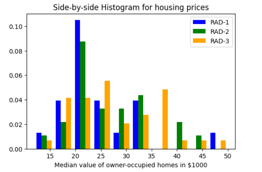
When you want to understand the distribution of data with respect to different characteristics, you could plot the side-by-side or multiple histograms on the same plot. For example, when you want to understand the distribution of housing prices with respect to different values of accessibility to radial highways, you would want to print the histograms side-by-side on the same plot. Here is the code representing the printing of histogram plots side-by-side on the same plot:
import pandas as pd
import numpy as np
from sklearn import datasets
import matplotlib.pyplot as plt
import matplotlib
%matplotlib inline
matplotlib.rcParams['font.size'] = 10
matplotlib.rcParams['figure.dpi'] = 100
from IPython.core.pylabtools import figsize
# Load boston housing price dataset
housing_prices = datasets.load_boston()
# Create Pandas dataframe
hp_data_transpose = housing_prices.data.transpose()
df_hp = pd.DataFrame({
  'CRIM': hp_data_transpose[0],
  'ZN':hp_data_transpose[1],
  'INDUS':hp_data_transpose[2],
  'CHAS':hp_data_transpose[3],
  'NOX':hp_data_transpose[4],
  'RM':hp_data_transpose[5],
  'AGE':hp_data_transpose[6],
  'DIS':hp_data_transpose[7],
  'RAD':hp_data_transpose[8],
  'TAX':hp_data_transpose[9],
  'PTRATIO':hp_data_transpose[10],
  'B':hp_data_transpose[11],
  'LSTAT':hp_data_transpose[12]
})
df_hp['MEDV'] = housing_prices.target
# Create histogram on MEDV column (target column)
figsize(6, 4)
# Create list of data according to different accessibility index
#
x1 = list(df_hp[df_hp['RAD'] == 1]['MEDV'])
x2 = list(df_hp[df_hp['RAD'] == 2]['MEDV'])
x3 = list(df_hp[df_hp['RAD'] == 3]['MEDV'])
# Setting colors and names
#
colors=['blue', 'green', 'orange']
names=['RAD-1', 'RAD-2', 'RAD-3']
# Creating plot with list values, colors and names (labels)
# Note the density value set as true which represents the
# probability distribution
#
plt.hist([x1, x2, x3], color=colors, label=names, density=True)
# Set the legend and labels
#
plt.legend()
plt.title('Side-by-side Histogram for housing prices')
plt.xlabel('Median value of owner-occupied homes in $1000')
Here is how the side-by-side histogram plot would look like:
Creating Stacked Histogram Plots using Matplotlib & Pandas
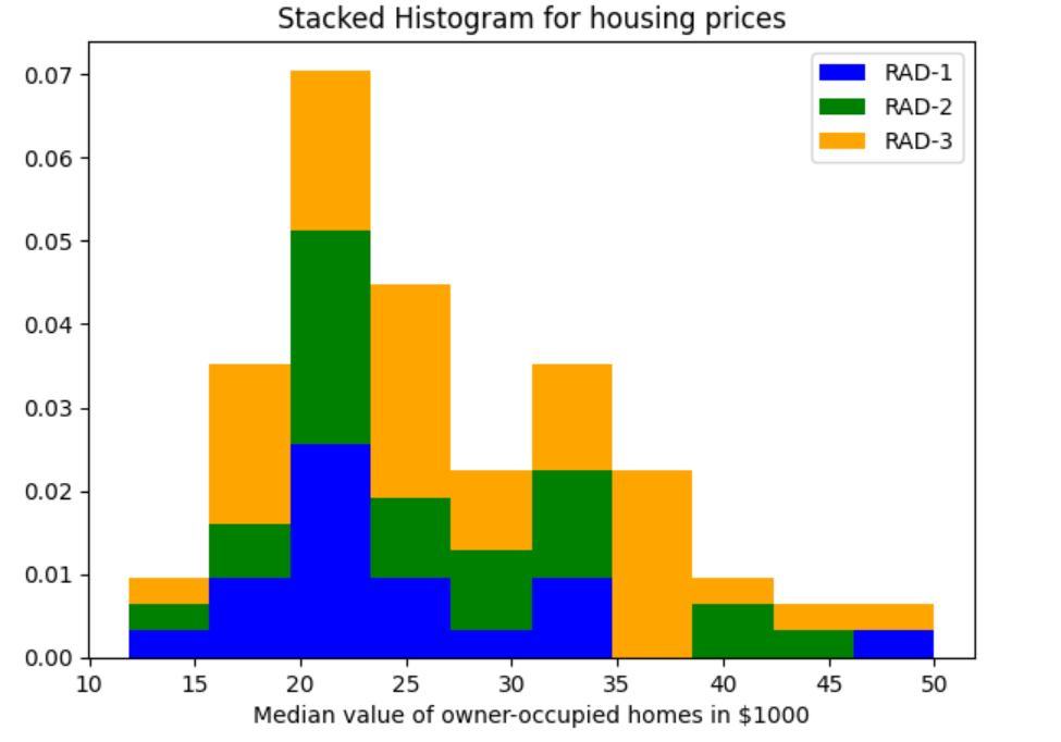
Another requirement can be to view the histogram plots stacked over each other. The requirement is to understand the data distribution against different attribute values while having the plots stacked over each other. This is different from side-by-side histogram in the way that the plots are stacked over each other. The difference in the code will only be an addition of another parameter, stacked = True in the plot function code used to draw side-by-side multiple histogram plots. Note the same in the code given below:
import pandas as pd
import numpy as np
from sklearn import datasets
import matplotlib.pyplot as plt
import matplotlib
%matplotlib inline
matplotlib.rcParams['font.size'] = 10
matplotlib.rcParams['figure.dpi'] = 100
from IPython.core.pylabtools import figsize
# Load boston housing price dataset
housing_prices = datasets.load_boston()
# Create Pandas dataframe
hp_data_transpose = housing_prices.data.transpose()
df_hp = pd.DataFrame({
  'CRIM': hp_data_transpose[0],
  'ZN':hp_data_transpose[1],
  'INDUS':hp_data_transpose[2],
  'CHAS':hp_data_transpose[3],
  'NOX':hp_data_transpose[4],
  'RM':hp_data_transpose[5],
  'AGE':hp_data_transpose[6],
  'DIS':hp_data_transpose[7],
  'RAD':hp_data_transpose[8],
  'TAX':hp_data_transpose[9],
  'PTRATIO':hp_data_transpose[10],
  'B':hp_data_transpose[11],
  'LSTAT':hp_data_transpose[12]
})
df_hp['MEDV'] = housing_prices.target
# Create histogram on MEDV column (target column)
figsize(7, 5)
# Create list of data according to different accessibility index
#
x1 = list(df_hp[df_hp['RAD'] == 1]['MEDV'])
x2 = list(df_hp[df_hp['RAD'] == 2]['MEDV'])
x3 = list(df_hp[df_hp['RAD'] == 3]['MEDV'])
# Setting colors and names
#
colors=['blue', 'green', 'orange']
names=['RAD-1', 'RAD-2', 'RAD-3']
# Creating plot with list values, colors and names (labels)
# Note the density value set as true which represents the
# probability distribution
# Note the parameter stacked = True which results in stacked histogram plot
#
plt.hist([x1, x2, x3], color=colors, label=names, density=True, stacked = True)
# Set the legend and labels
#
plt.legend()
plt.title('Stacked Histogram for housing prices')
plt.xlabel('Median value of owner-occupied homes in $1000')
The stacked histogram plot would look like the following:
We hope you found this introduction to histogram plots helpful along with how to create histogram plots using Matplotlib and Pandas packages in Python. If you have any questions, please don’t hesitate to reach out to us. And be sure to check out our other tutorials for more in-depth looks at data science and Python programming.

Check out my latest book titled as First Principles Thinking: Building winning products using first principles thinking.
- Three Approaches to Creating AI Agents: Code Examples - June 27, 2025
- What is Embodied AI? Explained with Examples - May 11, 2025
- Retrieval Augmented Generation (RAG) & LLM: Examples - February 15, 2025
I found it very helpful. However the differences are not too understandable for me