Last updated: 5th Dec, 2023
Regression analysis is a fundamental statistical technique used in many fields, from finance, econometrics to social sciences. It involves creating a regression model for modeling the relationship between a dependent variable and one or more independent variables. The Ordinary Least Squares (OLS) method helps estimate the parameters of this regression model.
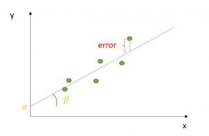
Ordinary least squares (OLS) is a technique used in linear regression model to find the best-fitting line for a set of data points by minimizing the residuals (the differences between the observed and predicted values). It does so by estimating the coefficients of the linear regression model by minimizing the sum of the squared differences between the observed values of the dependent variable and the predicted values from the model. It is a popular method because it is easy to use and produces decent results.
In this blog post, we will discuss the concepts and applications of the OLS method. We will explore how OLS method works, and its assumptions. We will also provide examples of how OLS can be used in different scenarios, from simple linear regression to more complex models. As data scientists, it is very important to learn the concepts of OLS before using it in the regression model.
What’s Ordinary Least Squares (OLS) Method in Machine Learning?
The ordinary least squares (OLS) method can be defined as a linear regression technique that is used to estimate the unknown parameters in a model. The OLS method minimizes the sum of squared residuals (SSR), defined as the difference between the actual (observed values of the dependent variable) and the predicted values from the model. The Ordinary Least Squares (OLS) method achieves the minimization of the Sum of Squared Residuals (SSR) by optimizing the values of the coefficients in a regression model so that the total of the squares of the differences between the observed values and the values predicted by the model is as small as possible. The resulting line representing the dependent variable of the linear regression model is called the regression line. This regression line represents the best fit for the data.
Ordinary Least Squares Formula – How to Calculate OLS
In mathematical terms, the OLS formula can be written as the following:
Minimize ∑(yi – ŷi)^2
where yi is the actual value, ŷi is the predicted value. A linear regression model used for determining the value of the response variable, ŷ, can be represented as the following equation.
y = b0 + b1x1 + b2x2 + … + bnxn + e
where:
- y is the dependent variable
- b0 is the intercept
- b1, b2, …, bn are the coefficients of the independent variables x1, x2, …, xn
- e is the error term
The coefficients b1, b2, …, bn can also be called the coefficients of determination. The goal of the OLS method can be used to estimate the unknown parameters (b1, b2, …, bn) by minimizing the sum of squared residuals (SSR). The sum of squared residuals is also termed the sum of squared error (SSE).
This method is also known as the least-squares method for regression or linear regression.
Assumptions of OLS Method
The OLS method relies on several assumptions to be valid. The following is the list of key assumptions:
- Linearity: There must be linear relationship between the dependent variable and the independent variables.
- Independence: The observations must be independent of each other.
- Homoscedasticity: The variance of the residuals should be constant across all levels of the independent variables.
- Normality: The residuals / errors should be normally distributed.
- No multicollinearity: The independent variables should not be highly correlated with each other.
Minimizing the Sum of Squares Residuals in OLS Method
The following represents the calculus method for minimizing the sum of squares residuals to find the unknown parameters for the model y = mx + b
Take the partial derivative of the cost function, sum of squared residuals, ∑(yi – ŷi)^2 with respect to m:
∂/∂m (SSE) = ∑-2Xi(yi – ŷi)
Take the partial derivative of the cost function, ∑ (yi – ŷi)^2 with respect to b:
∂/∂b (SSE) = ∑-2(yi – ŷi)
Set the partial derivatives equal to zero and solve for m and b:
∑-2Xi(yi – ŷi) = 0
∑-(yi – ŷi) = 0
This results in the following two equations:
∑yi*xi = m∑xi*xi + b*∑xi
∑yi = m∑xi + b*n
where n is the number of data points. These two equations can be solved simultaneously to find the values for m and b. Let’s say that the following three points are available such as (3, 7), (4, 9), (5, 12). And, the ask is to find the best fit line.
We will apply the calculus technique and use the above formulas. We will use the following formula:
∑-2Xi(yi – ŷi) = 0
The following calculation will happen:
-2[3(7 – (3m + b)) + 4(9 – (4m + b)) + 5(12 – (5m + b))] = 0
=> 3*7 + 4*9 + 5*12 – (9m + 3b + 16m + 4b + 25m + 5b) = 0
=> 21 + 36 + 60 – (50m + 12b) = 0
=> 116 = 50m + 12b …. eq (1)
Let’s use another formula to find another equation:
∑-(yi – ŷi) = 0
The following calculation will happen:
7 – (3m + b) + 9 – (4m + b) + 12 – (5m + b) = 0
=> 28 = 12m + 3b … eq(2)
The above two equations can be solved and the values of m and b can be found.
Evaluating OLS Results
OLS provides us with estimates of the coefficients of a linear regression model, but it’s important to evaluate how well the model fits the data. In this section, we will discuss different methods for evaluating OLS results such as some of the following:
- Residual analysis
- R-squared and adjusted R-squared
- F-statistics
Residual Analysis
Residual analysis involves examining the residuals (the differences between the observed values of the dependent variable and the predicted values from the model) to assess how well the model fits the data. Ideally, the residuals should be randomly scattered around zero and have constant variance.
If the residuals exhibit a pattern (such as a U-shape or a curve), it suggests that the model may not be capturing all of the relevant information. In this case, we may need to consider adding additional variables or transforming the data.
R-squared and Adjusted R-squared
R-squared is a measure of how much of the variation in the dependent variable is explained by the independent variables in the model. It ranges from 0 to 1, with higher values indicating a better fit.
Adjusted R-squared is similar to R-squared, but it takes into account the number of independent variables in the model. It is a more conservative estimate of the model’s fit, as it penalizes the addition of variables that do not improve the model’s performance.
F-Statistic
The F-statistic in linear regression model tests the overall significance of the model by comparing the variation in the dependent variable explained by the model to the variation not explained by the model. A large F-statistic indicates that the model as a whole is significant.
Alternative Methods to OLS
While OLS is a popular method for estimating linear regression models, there are several alternative methods that can be used depending on the specific requirements of the analysis. Let’s discuss some of the popular alternative methods to OLS.
- Ridge regression
- Lasso regression
- Elastic net regression
Ridge Regression
Ridge regression is a method that adds a penalty term to the OLS cost function to prevent overfitting in scenarios where there are many independent variables or the independent variables are highly correlated. The penalty term, known as the shrinkage parameter, reduces the magnitude of the coefficients and can help prevent the model from being too complex.
Lasso Regression
Lasso regression is similar to ridge regression, but it adds a penalty term that can result in some of the coefficients being set to zero. This can help simplify the model and reduce the risk of overfitting.
Elastic Net Regression
Elastic net regression is a combination of ridge and lasso regression that adds both a L1 and L2 penalty term to the OLS cost function. This method can help balance the advantages of both methods and can be particularly useful when there are many independent variables with varying degrees of importance.
Frequently Asked Questions (FAQs) for OLS Method
The following are some of the FAQs related to OLS method:
- How is ordinary least square method used in econometrics?
- In econometrics, the Ordinary Least Squares (OLS) method is crucial for estimating linear relationships between variables, constructing predictive models, and testing economic theories. It’s instrumental in policy analysis, helping evaluate the impacts of decisions like tax changes. OLS is valued for its data efficiency and ability to provide unbiased estimators under certain conditions. It also plays a key role in error analysis, addressing issues like heteroskedasticity and autocorrelation. While primarily used in time series analysis, OLS is equally effective with cross-sectional and panel data, making it a fundamental tool in the field of econometrics.
- What are some real-world examples where ordinary least squares method is used?
- Ordinary Least Squares (OLS) is used across various fields for analyzing relationships and making predictions. In economics, it’s employed to examine factors influencing GDP growth, like investment and labor. Real estate analysts use OLS to predict house prices based on size, location, and age. Marketing teams apply it to assess the impact of different advertising strategies on sales. In healthcare, OLS helps analyze how lifestyle choices affect health outcomes, such as the impact of exercise on blood pressure. Educational researchers use it to study the factors affecting student performance, including study hours and socio-economic status. Labor economists might employ OLS to understand the determinants of wages, considering education and experience.
Summary
The ordinary least squares (OLS) method in statistics is a technique that is used to estimate the unknown parameters in a linear regression model. The method relies on minimizing the sum of squared residuals between the actual and predicted values. The OLS method can be used to find the best-fit line for data by minimizing the sum of squared errors or residuals between the actual and predicted values. And, the calculus method for minimizing the sum of squares residuals is take the partial derivative of the cost function with respect to the coefficients of determination, set the partial derivatives equal to zero and solve for each of the coefficients. The OLS method is also known as least squares method for regression or linear regression.

Check out my latest book titled as First Principles Thinking: Building winning products using first principles thinking.
- Three Approaches to Creating AI Agents: Code Examples - June 27, 2025
- What is Embodied AI? Explained with Examples - May 11, 2025
- Retrieval Augmented Generation (RAG) & LLM: Examples - February 15, 2025
Why sum of squared residuals are taken?