Neural networks are an important part of machine learning, so it is essential to understand how they work. A neural network is a computer system that has been modeled based on a biological neural network comprising neurons connected with each other. It can be built to solve machine learning tasks, like classification and regression problems. The perceptron algorithm is a representation of how neural networks work. The artificial neurons were first proposed by Frank Rosenblatt in 1957 as models for the human brain’s perception mechanism. This post will explain the basics of neural networks with a perceptron example. You will understand how a neural network is built using perceptrons. This is a very important concept in relation to getting a good understanding of deep learning. You will also learn related Tensorflow / Keras code snippets.
Here are the key concepts related to how a deep neural network is built using one or more perceptrons:
What is a Perceptron?
A perceptron is the most fundamental unit which is used to build a neural network. A perceptron resembles a neuron in the human brain. In the case of a biological neuron, multiple input signals are fed into a neuron via dendrite, and an output signal is fired appropriately based on the strength of the input signal and some other mechanism. The diagram below represents how input signals pass through the biological neuron.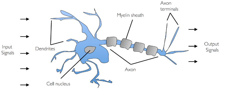
In the case of a perceptron, the input signals are combined with different weights and fed into the artificial neuron or perceptron along with a bias element. Representationally, within perceptron, the net sum is calculated as the sum of weights and input signal, and a bias element, then, the net sum is fed into a non-linear activation function. Based on the activation function, the output signal is sent out. The diagram below represents a perceptron. Notice the bias element b and sum of weights and input signals represented using x and w. The threshold function represents the non-linear activation function.
A perceptron can also be called a single-layer neural network as it is the part of the only layer in the neural network where the computation occurs. The computation occurs on the summation of input data that is fed into it. To understand greater details around perceptron, here is my post – Perceptron explained with Python example. The way that Rosenblatt Perceptron differed from McCulloch-Pitts Neuron (1943) is that in the case of Perceptron, the weights were learned based on the input data pertaining to different categories.
The perceptrons laid out in form of single-layer or multi-layer neural networks can be used to perform both regression and classification tasks. The diagram below represents the single-layer neural network (perceptron) that represents linear regression (left) and softmax regression (each output o1, o2, and o3 represents logits). Recall that the Softmax regression is a form of logistic regression that normalizes an input value into a vector of values that follows a probability distribution whose total sums up to 1. The output values are in the range [0,1]. This allows the neural network to predict as many classes or dimensions as required. This is why softmax regression is sometimes referred to as a multinomial logistic regression.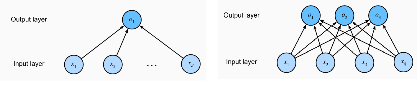
Here is a picture of a perceptron represented as the sum of the summation of inputs with weights (w1, w2, w3, wm) and bias element, that is passed through the activation function and the final output is obtained. This can be very well used for both regression and binary classification problems.
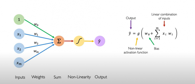
Fig. Perceptron
Here is an example of a multi-output perceptron. Note that perceptron is stacked and there are two outputs. Also, note that the perceptrons are fully connected, e.g., each output is connected with every input through perceptrons. The layers consisting of perceptrons that are connected to all inputs are called dense layers or fully connected layers. The dense layer is also called a stack of perceptrons. A configuration such as the one given below having multiple output neurons can be used to solve multi-class classification problems.
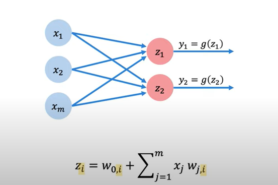
Fig. Multi-output perceptron
The above dense layer consisting of two units can be represented using the following TensorFlow code:
import tensorflow as tf
layer = tf.keras.layer.Dense(units = 2)
What is a deep neural network (DNN)?
A deep neural network (DNN) can be said to represent the mathematical model of the human brain. As the human brain is made up of a large number of neurons, a deep neural network is also made up of a large number of neuron-like units called perceptrons. A deep neural network is called “deep” because multiple levels of composition are learned. The multiple levels of composition can also be understood as representations that are used for predictions. The perceptron in the deep neural network is laid out in form of four or more layers including one input layer, one output layer, and one or more hidden layers. Note that the actual computations happen in the hidden and output layers. Thus, a deep neural network comprises two or more layers with each layer consisting of one or more perceptrons.
A neural network consisting of one or more hidden layers, and an output layer is commonly known as a multi-layer perceptron (MLP) neural network. The multi-layer perceptron network is a fully-connected neural network as each perceptron unit is fed inputs from all the units in the previous layer and the output from each perceptron is fed into each of the different neuron units in the next layer. Here is an example of fully connected multi-layer perceptron used to classify whether the person in an image is smiling.

In the above multi-layer perceptron neural network, the following happens:
- In first layer, the input image is fed in form of pixels
- In second layer, the input pixels combine to form low-level features such as edges
- In third layer, the low-layer features are combined and each of the nodes / units get fired when a high-level features such as eyes or nose or teeth are seen in the image.
- In the final layer, the high level features are combined and the nodes get fired when the person found in the image is seen to be smiling.
How does multi-layer perceptron work?
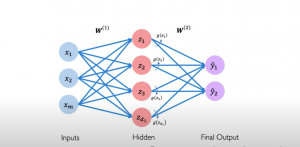
This is how the input flows through the multi-layer perceptron (MLP) network. The input comprising of one or more inputs combined with weights and along with a bias element is fed into each perceptron of the first hidden layer. For each of the perceptrons, the weights can be different. The output from the perceptrons in the first hidden layer is combined with new weights and fed into each perceptron of the second hidden layer along with a bias element and so on and so forth until the final output layer is reached. Note that weights combined with input to different perceptrons can be different. Such layers where all perceptrons are connected with all inputs combined with different weights are also termed dense layers. And, the neural network with dense layers is called a fully connected neural network. Refer to the picture given below showing a multi-layer perceptron neural network comprising one hidden layer and one output layer. Note that each layer will have its own set of weights. Also, z1, z2, z3, and z4 represent net input which is the sum of weights and inputs. In the neural network shown below, there are 4 perceptrons in the hidden layer and 2 perceptrons in the output layer. Each of the perceptrons will have an associated non-linear activation function represented using the letter g. When there is two or more hidden layer, such neural networks are called a deep neural network. And, the learning is called deep learning. In the picture below, a multi-layer perceptron (MLP) neural network is shown.
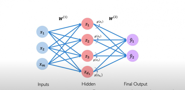
Fig 1. Multi-layer perceptron (MLP) neural network
In the picture below, note how net input is calculated as a sum of input signals and weights.
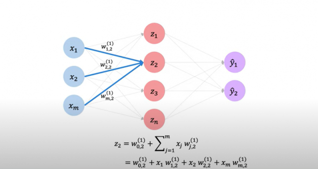
Fig 2. Neural network – Net input explained
The above can be represented as a sequential neural network with two layers (hidden and output layer) in TensorFlow using the following code:
import tensorflow as tf

model = tf.keras.Sequential([
    tf.keras.layers.Dense(units=n),
    tf.keras.layers.Dense(units=2)
])

# Above code can also be written as the following:
model = tf.keras.Sequential([
    tf.keras.layers.Dense(n),
    tf.keras.layers.Dense(2)
])
In the above code, the first layer is a dense layer having n units, and the second layer, which is also the output layer, is a dense layer having two units.
In case, there are 5 dense layers with 4 hidden and 1 output layer with n1 unit in the first layer, n2 in the second layer, n3 in the third layer, n4 in the 4th layer, and 3 units in the last layer, the model code in TensorFlow would look like the following:
import tensorflow as tf

model = tf.keras.Sequential([
    tf.keras.layers.Dense(n1),
    tf.keras.layers.Dense(n2),
    tf.keras.layers.Dense(n3),
    tf.keras.layers.Dense(n4),
    tf.keras.layers.Dense(3)
])
An example of a Neural Network using Tensorflow / Keras
Here is a screenshot for a simple piece of code to train an artificial neural network that can be used to identify different class of images:
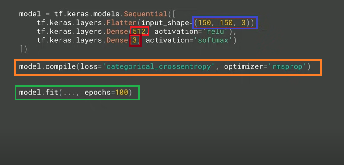
Fig 3. Understanding artificial neural networks using Tensorflow and Keras
There are five important concepts to learn in the above Tensorflow code. They are as follows:
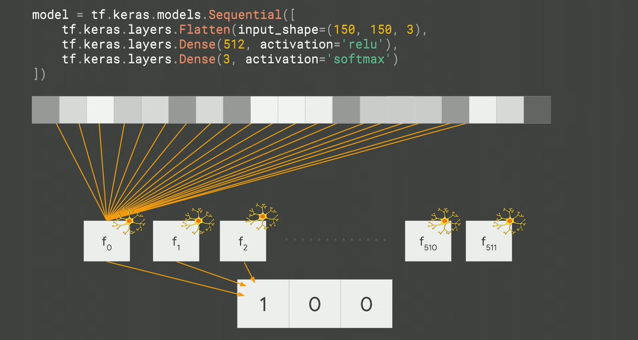
- The blue color box represents the input image of size 150 x 150 with 3-bit color depth
- The brown color box represents the output which are three different classes that neural networks with classifying any image.
- The red color box represents 512 which, simply speaking, are 512 functions with each function having its own internal variables. The boxes in the diagram below represent these 512 functions. These 512 functions (also called neurons – see the diagram below) are fed with image pixels and trained based on the given label or output as 1 for the actual class. Machine learning is about identifying those internal variables (also called parameters) in different neurons (512 functions) to match the desired output (given label). The activation function used for each of the internal functions is ReLU.
- In the beginning of the training, these 512 functions’ parameters are initialized with some random values. How do these parameters’ values get adjusted during training purpose. This is where the orange box comes into the picture. The categorical_crossentropy represents the loss function that calculates loss during training. The optimizer, rmsprop adjusts the value of parameters to decrease the loss after each iteration of training.
- Finally, epochs (green box) represent the number of iterations for training to happen.
The above can also be understood with the following diagram:
In this blog post, we’ve shared a brief overview of neural networks and how they work. We also took the time to walk through an example model using TensorFlow and Keras to show you just how easy it can be to train your own neural network with Python! If you want more information about these topics or if you are interested in learning more about machine learning or data science, reach out to us today. Our team is ready to provide expert mentorship so that you can get started right away using artificial intelligence in your business. What questions do you have about the artificial neural network? Let me know in the comments below and I will try and answer them at their earliest convenience!

Check out my latest book titled as First Principles Thinking: Building winning products using first principles thinking.
- Questions to Ask When Thinking Like a Product Leader - July 3, 2025
- Three Approaches to Creating AI Agents: Code Examples - June 27, 2025
- What is Embodied AI? Explained with Examples - May 11, 2025
I found it very helpful. However the differences are not too understandable for me