Artificial Neural Networks (ANN) have emerged as a powerful tool in machine learning, and Multilayer Perceptron (MLP) is a popular type of ANN that is widely used in various domains such as image recognition, natural language processing, and predictive analytics. Keras is a high-level API that makes it easy to build and train neural networks, including MLPs.
In this blog, we will dive into the world of MLPs and explore how to build and train an MLP model using Keras. We will build a simple MLP model using Keras and train it on a dataset. We will explain different aspects of training MLP model using Keras. By the end of this blog, you will have a good understanding of how to implement MLPs using Keras, which will help you to build more sophisticated and accurate neural network models in the future.
Before getting ahead into this blog, you would want to learn about detailed representation of multilayer perceptron (MLP) in this blog – Neural networks & Multilayer Perceptron: Examples.
Keras Code: Training Multilayer Perceptron Neural Network
The MLP model consists of multiple layers of interconnected neurons, where each neuron is connected to all the neurons in the previous and next layer. In the code below, we will work with MLP used for image classification that has four layers such as the following:
- The input layer: The input layer receives the input data.
- A flatten layer: The input data is flattened to a single dimension using the flatten layer. For the data used in the example, every image is represented using 32 x 32 x 3. Thus, when flattened, there will be 3072 entries representing all the pixels of each of the image.
- Two dense layers with Relu activation function: The two dense layers use the rectified linear unit (ReLU) activation function, which is commonly used in deep learning models due to its ability to handle non-linearity and avoid the vanishing gradient problem.
- One dense layer with softmax activation function: The final dense layer uses the softmax activation function, which is commonly used in multi-class classification problems to convert the output of the model into probabilities that sum up to one
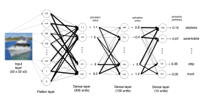
The training image data is fed as input to the input layer in form of tensor of shape, [50000, 32, 32, 3]. In the training dataset, the number 50000 refers to the total number of images in the dataset. The dimensions of each image are 32×32 pixels, and there are three color channels (red, green, and blue) for each pixel. Therefore, the shape of the training dataset is [50000, 32, 32, 3]. In other words, the training dataset is a 4D tensor with 50000 images, each having a height and width of 32 pixels, and 3 color channels. The shape of the test data set tensor is [10000, 32, 32, 3]. There are 10000 images of size 32×32 with 3 color channels (RGB). There are 10 classes that images need to be classified. The following is a visual representation of the image. The numbers at every unit in the two dense layers represents the summation of weights and input from all the units in the previous layer. There are 200 units in one dense layer and 150 units in another dense layer. This is why the layers are called dense.

The following are important steps to training multilayer perceptron neural network. We will go through each of the step while writing the code using Keras.
- Prepare the data: Prepare the data that you will use to train the MLP. This typically involves splitting the data into training and testing sets, as well as preprocessing the data as necessary (e.g., scaling the features, one-hot encoding the labels).
- Define the model architecture: Define the architecture of the MLP, specifying the number and type of layers, the activation functions, the number of units in each layer, and any other relevant hyperparameters.
- Compile the model: Compile the MLP, specifying the loss function, the optimizer, and any relevant metrics.
- Train the model: Train the MLP on the training data, specifying the number of epochs and batch size.
- Evaluate the model: Evaluate the performance of the MLP on the test data, calculating any relevant metrics (e.g., accuracy, precision, recall, F1 score).
- Visualize the results: Visualize the performance of the MLP during training, using plots of the training and validation loss and accuracy.
Preparing the Data for Training MLP Network
is the first important step to training a multilayer perceptron neural network using Keras. This step involves loading and preparing the data that we will use to train the MLP network.
Pixel scaling is an important preprocessing step that is often applied to the input data. In machine learning, it is common to scale the features to a range between 0 and 1 to make them easier to work with. In image classification tasks, the pixel values in the images can range from 0 to 255 (for 8-bit images). Scaling the pixel values to be between 0 and 1 can make the model training process more stable and efficient. This can be done by dividing each pixel value by 255.
One-hot encoding is a way of representing categorical data as binary vectors. In classification tasks, the output labels are often categorical, meaning they belong to a fixed set of classes. One-hot encoding is used to convert these categorical labels into vectors of 0s and 1s. Each vector has the same length as the number of classes, and the value at the index corresponding to the true class is set to 1, while all other values are set to 0. This is necessary because the model’s output layer usually produces a probability distribution over the classes, and one-hot encoding makes it easy to compare the predicted probabilities to the true labels. Keras provides a utility function called to_categorical to convert the labels to one-hot encoding.
from tensorflow.keras.datasets import cifar10
from tensorflow.keras.utils import to_categorical

# Load the CIFAR-10 dataset
(x_train, y_train), (x_test, y_test) = cifar10.load_data()

# Scale the pixel values to between 0 and 1
x_train = x_train / 255.0
x_test = x_test / 255.0

# Convert the labels to one-hot encoding
y_train = to_categorical(y_train)
y_test = to_categorical(y_test)
Defining the MLP Model Architecture
There are two ways to define the structure of a neural network in Keras, They are as following:
- Using sequential model
- Using the Functional API.
Here’s an explanation for each one of the above approachs and code examples for creating a multilayer perceptron (MLP) with a 32x32x3 input and 10 outputs.
Keras Sequential Model Structure for MLP
The Sequential model is a linear stack of layers, where you can easily add new layers to the model. You can create a Sequential model by calling the Sequential class and then adding layers to it using the add method. Here’s the code for creating an MLP with two dense layers of 200 and 150 units each and a softmax output layer:
from tensorflow.keras.models import Sequential
from tensorflow.keras.layers import Dense, Flatten
# Create a Sequential model
model = Sequential()
# Add a Flatten layer to flatten the input image
model.add(Flatten(input_shape=(32, 32, 3)))
# Add two dense layers with 200 units and 'relu' activation function
model.add(Dense(200, activation='relu'))
model.add(Dense(150, activation='relu'))
# Add a softmax output layer with 10 units
model.add(Dense(10, activation='softmax'))
# Print the model summary
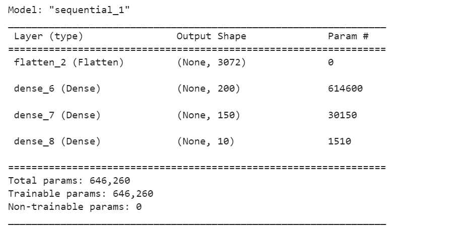
model.summary()
The following is what will get printed.
Keras Functional API Model Structure for MLP
The Functional API allows you to define more complex models, including models with multiple inputs or outputs or models with shared layers. To use the Functional API, you first define the input layer and then create a chain of layers by calling them on the input layer. Here’s the code for creating an MLP with two dense layers of 200 and 150 units and a softmax output layer using the Functional API:
from tensorflow.keras.layers import Input, Dense, Flatten
from tensorflow.keras.models import Model

# Define the input layer
inputs = Input(shape=(32, 32, 3))

# Flatten the input image
x = Flatten()(inputs)

# Add two dense layers with 200 units and 'relu' activation function
x = Dense(200, activation='relu')(x)
x = Dense(150, activation='relu')(x)

# Add a softmax output layer with 10 units
outputs = Dense(10, activation='softmax')(x)

# Create the model
model = Model(inputs=inputs, outputs=outputs)

# Print the model summary
model.summary()
This is how the model structure summary would look like:

Which of the Model Structure to use: Sequential or Functional API
The Functional API method in Keras is recommended for creating more complex models that have multiple inputs, multiple outputs, or require layers to share connections. The Sequential model, on the other hand, is suitable for creating simple models where the layers are stacked linearly.
Many deep learning models require that the output from a layer is passed to multiple subsequent layers, or conversely, that a layer receives input from multiple preceding layers. For example, a network with skip connections or residual connections would require the output from one layer to be fed directly to a later layer, bypassing some intermediate layers. In such cases, the Sequential class would not be suitable for defining the model structure. The Functional API allows for more flexibility in defining the structure of the model, enabling the creation of complex models with multiple inputs, outputs, or shared layers.
Therefore, if you need to create a model with complex structure, it is recommended to use the Functional API in Keras.
Compile the MLP Model
Compiling a model in Keras involves configuring the model’s learning process by specifying the optimizer, loss function, and evaluation metric.
from tensorflow.keras import optimizers

opt = optimizers.Adam(learning_rate=0.0005)
model.compile(loss='categorical_crossentropy', optimizer=opt, metrics=['accuracy'])
The following is the detail related to loss function, optimizer and metrics used in the above code:
- Loss function: In the case of a multiclass classification problem, the categorical cross-entropy loss function is commonly used. This loss function measures the difference between the predicted probabilities and the true class labels. The categorical cross-entropy loss is a good choice for multiclass classification problems as it takes into account the probability distribution of the output classes. For binary classification problem, binary cross entropy loss function is used and for regression problem, mean squared error loss function is used.
- Optimizer: Adam is a popular optimization algorithm used to update the weights of a neural network during training. It combines the benefits of two other optimization algorithms: AdaGrad and RMSProp. Adam is known for its efficiency and ability to converge quickly to a solution. It adapts the learning rate based on the momentum and variance of the gradients, allowing for a smooth and fast convergence. The code imports the
optimizersmodule from the Keras library. Then, an Adam optimizer is created with a learning rate of 0.0005 by callingoptimizers.Adam(learning_rate=0.0005). - Metrics: The metric used to evaluate the model’s performance during training and testing is accuracy. Accuracy measures the fraction of correctly classified samples over the total number of samples. It is a commonly used metric for classification problems, especially when the classes are balanced.
Train the MLP Model
GIven that the model has been defined and compiled, it is time to train the model. The code below represents how to train the model using Keras with the given configuration:
model.fit(x_train, y_train, batch_size = 32, epochs = 10, shuffle = True)
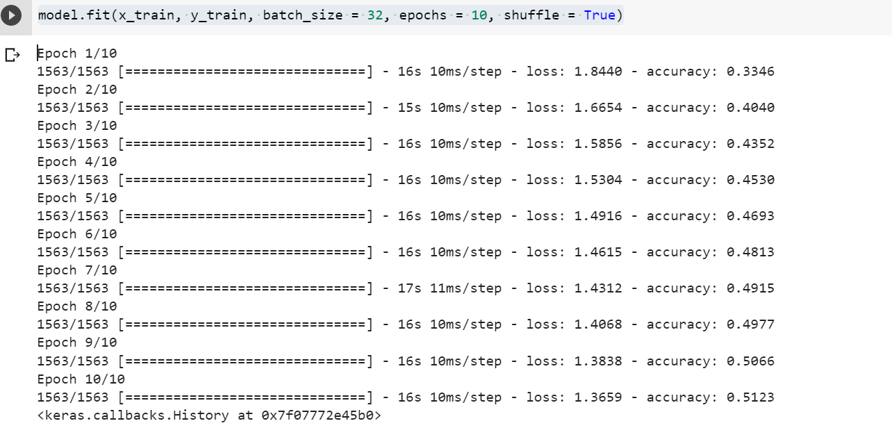
The fit() function in Keras is used to train the model on the given training data x_train and y_train. The batch_size parameter is set to 32, which means that the training data will be divided into batches of 32 samples each. The shuffle parameter is set to True, which means that the order of the training data will be shuffled before each epoch to prevent any bias that might be introduced due to the order of the samples.
The fit() function trains the model for a specified number of epochs set as 10. The model’s weights are updated after each batch of data is processed, and the process is repeated for the specified number of epochs = 10.
Evaluate the MLP Model
Finally, it is time to evaluate the multilayer perceptron model trained in the previous code. The following code is used to evaluate the model.
loss, accuracy = model.evaluate(x_test, y_test)
print('Test loss:', loss)
print('Test accuracy:', accuracy)
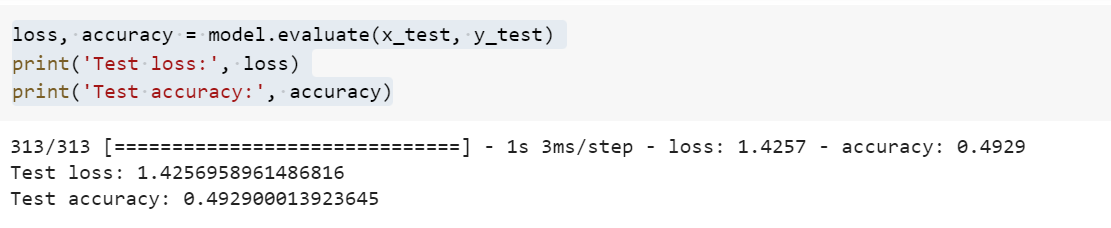
The evaluate() function in Keras is used to evaluate the performance of the model on the given test data x_test and y_test. The function returns the loss value and the metric value specified during the model compilation (in this case, accuracy).
The code above assigns the returned values to the loss and accuracy variables, and then prints them to the console. This provides a measure of how well the model performs on the test data.
Conclusion
In this blog, we have explored the steps required to build a Multilayer Perceptron (MLP) neural network using the Keras library. We started by preparing the data and then defining the architecture of the model.
We looked at two ways of defining the architecture of the MLP model in Keras – Sequential model structure and Functional API model structure. We also discussed the pros and cons of using each of these approaches.
After defining the model architecture, we compiled the model by specifying the loss function, optimizer, and evaluation metric. We then trained the model on the training data and evaluated its performance on the test data.
Keras provides a user-friendly interface for building MLP neural networks with just a few lines of code. By following the steps outlined in this blog, you can easily build your own MLP models for various machine learning tasks.

Check out my latest book titled as First Principles Thinking: Building winning products using first principles thinking.
- Mathematics Topics for Machine Learning Beginners - July 6, 2025
- Questions to Ask When Thinking Like a Product Leader - July 3, 2025
- Three Approaches to Creating AI Agents: Code Examples - June 27, 2025
I found it very helpful. However the differences are not too understandable for me