
In this post, you will learn about the concepts of Geometric probability distribution with the help of real-world examples and Python code examples. It is of utmost importance for data scientists to understand and get an intuition of different kinds of probability distribution including geometric distribution. You may want to check out some of my following posts on other probability distribution.
- Normal distribution explained with Python examples
- Binomial distribution explained with 10+ examples
- Hypergeometric distribution explained with 10+ examples
In this post, the following topics have been covered:
- Geometric probability distribution concepts
- Geometric distribution python examples
- Geometric distribution real-world examples
Geometric Probability Distribution Concepts
Geometric probability distribution is a discrete probability distribution. It represents the probability that an event having probability p will happen (success) after X number of Bernoulli trials with X taking values of 1, 2, 3, …k. A Bernoulli trial is a trial which results in either success or failure. Geometric distribution of random variable, X, represents the probability that an event will take X number of Bernoulli trials to happen. Here, X can be termed as discrete random variable. In other words, Geometric distribution is probability distribution of X trials represents the probability that there will be X – 1 failure before the event event occurs. Here the basic assumption is that the trials are independent of each other.
Mathematically, if p is the probability that the event occurs, then the probability that event will not occur is 1 – p. The probability that the event will happen after k trials can be represented in form of the following probability mass function.
[latex]\Large Pr(X = k) = (1-p)^{(k-1)}p[/latex]
.
Lets understand the concept in a more descriptive manner using basketball free throws shot example. In basketball, free throws or foul shots are unopposed attempts to score points by shooting from behind the free throw line (informally known as the foul line or the charity stripe), a line situated at the end of the restricted area. Let’s say that the players in the below picture is contesting as to how many shoots one will take to achieve a perfect throw (scoring a point). The goal is to find the probability that the shooter will have the first perfect throw in X number of shoots.

Let’s say the the shooter in the above picture has a probability of scoring the perfect throw is 0.6. So, the goal is to find out the probability that the shooter will have perfect throw in 1st throw, 2nd throw (1st throw as unsuccessful), third throw (1st two throws as unsuccessful), fourth throw (1st three throws as unsuccessful), fifth throw ((1st four throws as unsuccessful) etc. You may note that we may end up with probability distribution for random variable X representing the number of shoots a person will take to have first perfect throw.
Let’s calculate the probability of X = 1, 2, 3, 4, 5 number of throws for first successful throw. Given the probability of a perfect throw (success) is 0.6 and, thus, the probability of unsuccessful throw (failure) is 0.4 (1-0.6), here is how the probability distribution would look like for different values of X.
| X = (1, 2, 3..) | Probability calculation that the prefect throw happen in X | Net Probability |
| 1 | 0.6 | 0.6 |
| 2 | 0.4 x 0.6 ([latex]0.4^1*0.6[/latex]) | 0.24 |
| 3 | 0.4 x 0.4 x 0.6 ([latex]0.4^2*0.6[/latex]) | 0.096 |
| 4 | 0.4 x 0.4 x 0.4 x 0.6 ([latex]0.4^3*0.6[/latex]) | 0.0384 |
| … | … | … |
| k | 0.4 x 0.4 x 0.4 … 0.6 ([latex]0.4^{(k-1)}*0.6[/latex]) | [latex]0.4^{(k-1)}*0.6[/latex] |
You may note that the coefficients of X = k is k – 1.
Expectation and Variance of Geometric Distribution
The expectation of geometric distribution can be defined as expected number of trials in which the first success will occur. The mathematical formula to calculate the expected value of geometric distribution can be calculated as the following where p is probability that the event occur.
[latex]\Large \frac{1}{p}[/latex]
.
The variance of geometric distribution can be defined as variance of number of trials it may take for success to happen. Mathematically, variance can be calculated using the following:
[latex]\Large \frac{q}{p^2}[/latex]
.
Geometric Distribution Python Example
Here is the Python code calculating geometric probability distribution. Pay attention to some of the following:
- Discrete random variable X is defined along with probability of the perfect throw (event to occur)
- Scipy.stats geom class is used to calculate the probability mass function using the method, pmf.
from scipy.stats import geom
import matplotlib.pyplot as plt
#
# X = Discrete random variable representing number of throws
# p = Probability of the perfect throw
#
X = [1, 2, 3, 4, 5, 6, 7, 8, 9, 10]
p = 0.6
#
# Calculate geometric probability distribution
#
geom_pd = geom.pmf(X, p)
#
# Plot the probability distribution
#
fig, ax = plt.subplots(1, 1, figsize=(8, 6))
ax.plot(X, geom_pd, 'bo', ms=8, label='geom pmf')
plt.ylabel("Probability", fontsize="18")
plt.xlabel("X - No. of Throws", fontsize="18")
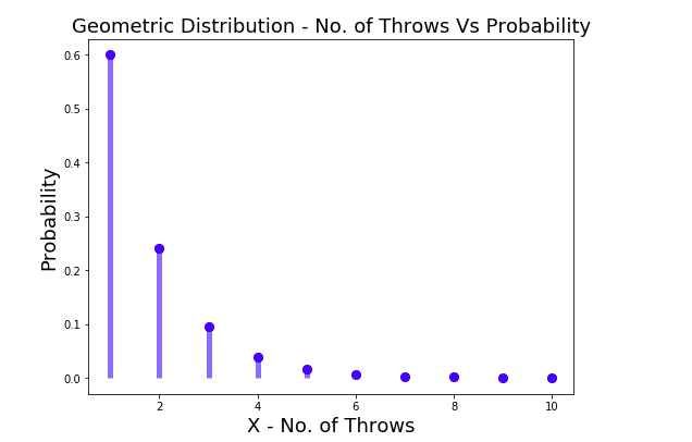
plt.title("Geometric Distribution - No. of Throws Vs Probability", fontsize="18")
ax.vlines(X, 0, geom_pd, colors='b', lw=5, alpha=0.5)
Here is the plot representing the geometric distribution for P = 0.6 and different values of X.
Geometric Distribution Real-world Examples
Here are some real-world examples of Geometric distribution with the assumption that the trials are independent of each other.
- Let’s say, the probability that an athlete achieves a distance of 6m in long jump is 0.7. Geometric distribution can be used to determine probability of number of attempts that the person will take to achieve a long jump of 6m. In the second attempt, the probability will be 0.3 * 0.7 = 0.21 and the probability that the person will achieve in third jump will be 0.3 * 0.3 * 0.7 = 0.063
- Here is another example. Let’s say the probability that the person climbs the hill without stopping anywhere is 0.3. Geometric distribution can be used to represent the probability of number of attempts that the person will take to climb the hill. The probability to achieve in first attempt is 0.3, second attempt is 0.7*0.3 = 0.21, third attempt is 0.7*0.7*0.3 = 0.147
Conclusions
Here is the summary of what you learned about the Geometric probability distribution:
- Geometric probability distribution is about determining probabilities of discrete random variable X which represents number of trials it would take for the event to happen (first time).
- The trials would need to be independent of each other.

Check out my latest book titled as First Principles Thinking: Building winning products using first principles thinking.
- Questions to Ask When Thinking Like a Product Leader - July 3, 2025
- Three Approaches to Creating AI Agents: Code Examples - June 27, 2025
- What is Embodied AI? Explained with Examples - May 11, 2025
I found it very helpful. However the differences are not too understandable for me