What is normal distribution? It’s a probability distribution that occurs in many real world cases. In this blog post, you will learn about the concepts of Normal Distribution with the help of Python example. As a data scientist, you must get a good understanding of different probability distributions in statistics in order to understand the data in a better manner. Normal distribution is also called as Gaussian distribution or Laplace-Gauss distribution.
Normal Distribution with Python Example
Normal distribution is the default probability for many real-world scenarios. It represents a symmetric distribution where most of the observations cluster around the central peak called as mean of the distribution. A normal distribution can be thought of as a bell curve or Gaussian Distribution which typically has two parameters: mean and standard deviation (SD). The parameter used to measure the variability of observations around the mean is called standard deviation. The probabilities for values occurring near the mean are higher than the values far away from the mean. The parameters of the normal distribution plot defining the shape and the probabilities are mean and standard deviation. The area of the plot between two different points in the normal distribution plot represents the probability of the value occurring between those two points.
Many machine learning algorithms assume normal distribution in the data. If you have normally distributed inputs, use a normal probability function to calculate the probability of their occurrence. If your inputs are not normally distributed, transform them by applying log or square root transformations until they become normally distributed before feeding them into an algorithm that assumes normal distribution (such as linear regression).
Here are some of the properties of the normal distribution of the population:
- The points in the normal distribution are symmetric. The normal distribution can not be used to model skewed distributions.
- The mean, median, and mode of the normal distribution are equal.
- Half of the population is less than the mean and half is greater than the mean.
- The empirical rule of the normal distribution goes like the following: 68% of the observations fall within +/- 1 standard deviation from the mean, 95% of the observations fall within +/- 2 standard deviation from the mean and 99.7% of the observations fall within +/- 3 standard deviations from the mean.
Here is the probability density function for normal distribution:
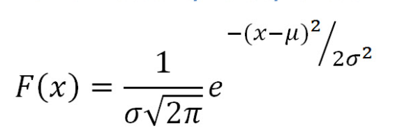
Fig 1. Normal distribution probability density function
In above function, [latex]\mu[/latex] represents the mean and [latex]\sigma[/latex] represents the standard deviation. Given different values of the random variable (x), one could calculate the probability using the above probability density function.
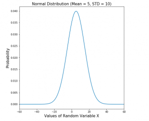
The technique to find whether data is normally distributed or otherwise is to draw a normal probability distribution plot. Here is a sample probability distribution plot representing normal distribution with a mean of 5 and a standard deviation of 10. The plot is created for random variables taking values between -100 and 100.
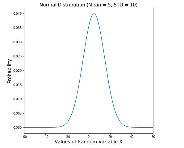
Fig 2. Normal Distribution Plot
The following code can be used to generate above normal distribution plot.
#
# Create a normal distribution with mean as 5 and standard deviation as 10
#
mu = 5
std = 10
snd = stats.norm(mu, std)
#
# Generate 1000 random values between -100, 100
#
x = np.linspace(-100, 100, 1000)
#
# Plot the standard normal distribution for different values of random variable
# falling in the range -100, 100
#
plt.figure(figsize=(7.5,7.5))
plt.plot(x, snd.pdf(x))
plt.xlim(-60, 60)
plt.title('Normal Distribution (Mean = 5, STD = 10)', fontsize='15')
plt.xlabel('Values of Random Variable X', fontsize='15')
plt.ylabel('Probability', fontsize='15')
plt.show()
Here is the code representing multiple normal distribution plots which looks like the following:
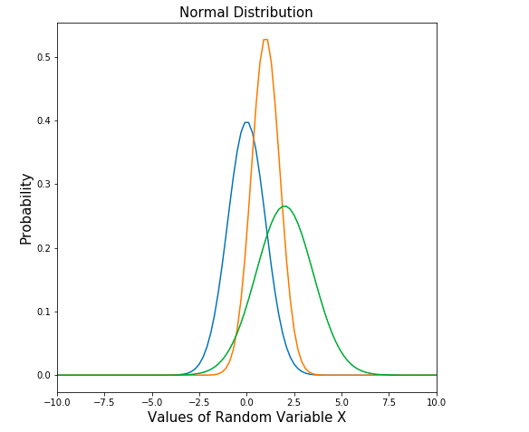
The following code can be used to create above shown multiple normal distribution plots having different means and standard deviation.
#
# Values of random variable
#
x = np.linspace(-10, 10, 100)
#
plt.figure(figsize=(7.5,7.5))
#
# Normal distribution with mean 0 and std as 1
#
plt.plot(x, stats.norm(0, 1).pdf(x))
#
# Normal distribution with mean 1 and std as 0.75
#
plt.plot(x, stats.norm(1, 0.75).pdf(x))
#
# Normal distribution with mean 2 and std as 1.5
#
plt.plot(x, stats.norm(2, 1.5).pdf(x))
plt.xlim(-10, 10)
plt.title('Normal Distribution', fontsize='15')
plt.xlabel('Values of Random Variable X', fontsize='15')
plt.ylabel('Probability', fontsize='15')
plt.show()
Standard Normal Distribution with Python Example
Standard Normal Distribution is the normal distribution with mean as 0 and standard deviation as 1.
Here is the Python code and plot for standard normal distribution. Note that the standard normal distribution has a mean of 0 and standard deviation of 1. Pay attention to some of the following in the code below:
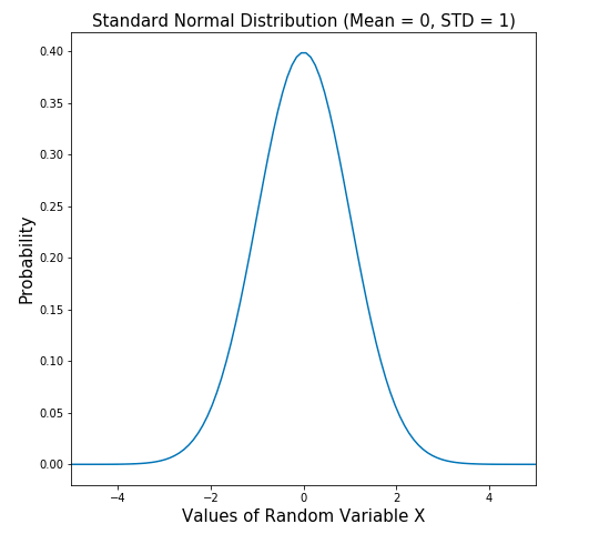
The following is the Python code used to generate the above standard normal distribution plot. Pay attention to some of the following in the code given below:
- Scipy Stats module is used to create an instance of standard normal distribution with mean as 0 and standard deviation as 1 (stats.norm)
- Probability density function pdf() is invoked on the instance of stats.norm to generate probability estimates of different values of random variable given the standard normal distribution
import numpy as np
import matplotlib.pyplot as plt
from scipy import stats
#
# Create a standard normal distribution with mean as 0 and standard deviation as 1
#
mu = 0
std = 1
snd = stats.norm(mu, std)
#
# Generate 100 random values between -5, 5
#
x = np.linspace(-5, 5, 100)
#
# Plot the standard normal distribution for different values of random variable
# falling in the range -5, 5
#
plt.figure(figsize=(7.5,7.5))
plt.plot(x, snd.pdf(x))
plt.xlim(-5, 5)
plt.title('Normal Distribution', fontsize='15')
plt.xlabel('Values of Random Variable X', fontsize='15')
plt.ylabel('Probability', fontsize='15')
plt.show()
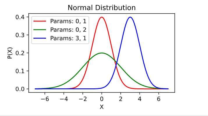
Even without using stats.norm.pdf function, we can create multiple normal distribution plots using the following Python code. Note the function normal (x, mu, sigma) and different pairs of mean and standard deviation parameters.
# Normal Distribution Function
#
def normal(x, mu, sigma):
    p = 1 / math.sqrt(2 * math.pi * sigma**2)
    return p * np.exp(-0.5 / sigma**2 * (x - mu)**2)

#
# Random variable X having different values
#
X = np.arange(-5, 5, 0.01)

# Mean, Standard deviation pairs
params = [(0, 1), (0, 2), (3, 1)]

#
# Plotting different normal distribution curves simultaneously
#
plt.plot(x, normal(x, params[0][0], params[0][1]), color='r', label='Params: 0, 1')
plt.plot(x, normal(x, params[1][0], params[1][1]), color='g', label='Params: 0, 2')
plt.plot(x, normal(x, params[2][0], params[2][1]), color='b', label='Params: 3, 1')

# Naming the x-axis, y-axis and the whole graph
#
plt.xlabel("X")
plt.ylabel("P(X)")
plt.title("Normal Distribution")

# Adding legend, which helps us recognize the curve according to it's color
plt.legend()

# To load the display window
plt.show()
Here is the plot created using the above code:
What are some real-world examples of normal distribution?
The real-world examples of the normal probability distribution are everywhere. Normal distributions apply to many situations in the real world including some of the following areas:
- Human heights (people of the same gender and age group typically cluster around average with normal distribution)
- IQ scores (the mean is typically 100, SD = 15)
- Marks of students in a class (mean = 60, SD = 20)
- Measure of weight (mean = 80 kg, SD = 10)
- Measure of blood pressure (mean = 120/80, SD = 20)
- Measure of distance (mean = 0, SD = 50)
- Time taken to complete a task (measurement in seconds; mean = 30 minutes, SD= 5 min.)
- Measure of wealth (measurement in money; mean = $50,000 , SD = $100)
- Height of trees (measurement in meters; mean = 40 m, SD = 20)
Conclusions
Here is the summary of what you learned in this post in relation to Normal distribution:
- Normal distribution is a symmetric probability distribution with equal number of observations on either half of the mean.
- The parameters representing the shape and probabilities of the normal distribution are mean and standard deviation
- Python Scipy stats module can be used to create a normal distribution with meand and standard deviation parameters using method norm.
- Standard normal distribution is normal distribution with mean as 0 and standard deviation as 1.
- In normal distribution, 68% of observations lie within 1 standard deviation, 95% of observations lie within 2 standard deviations and 99.7% observations lie within 3 standard deviations from the mean.

Check out my latest book titled as First Principles Thinking: Building winning products using first principles thinking.
- Mathematics Topics for Machine Learning Beginners - July 6, 2025
- Questions to Ask When Thinking Like a Product Leader - July 3, 2025
- Three Approaches to Creating AI Agents: Code Examples - June 27, 2025
I found it very helpful. However the differences are not too understandable for me