Have you ever wondered how to predict the number of successes in a series of independent trials? Or perhaps you’ve been curious about the probability of achieving a specific outcome in a sequence of yes-or-no questions. If so, we are essentially talking about the binomial distribution. It’s important for data scientists to understand this concept as binomials are used often in business applications.
The binomial distribution is a discrete probability distribution that applies to binomial experiments (experiments with binary outcomes). It’s the number of successes in a specific number of trials. Sighting a simple yet real-life example, the binomial distribution may be imagined as the probability distribution of a number of heads that appear on a coin flip in a specific experiment comprising of a fixed number of coin flips. In this blog post, we will learn binomial distribution with the help of examples. If you are an aspiring data scientist looking forward to learning/understand the binomial distribution in a better manner, this post might be very helpful.
What is a Binomial Distribution?
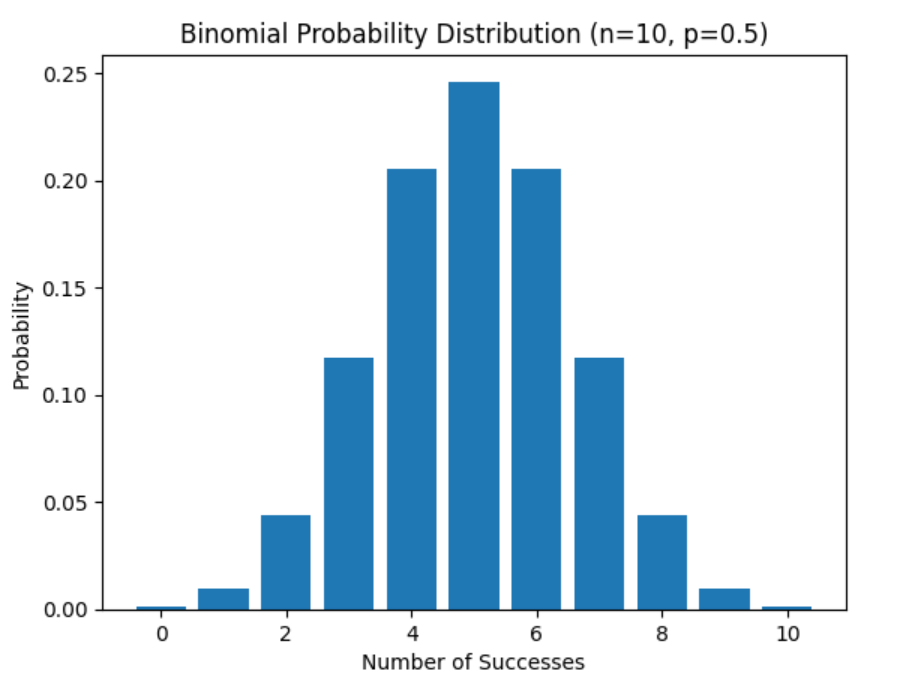
The binomial distribution is a discrete probability distribution that represents the probabilities of binomial random variables in a binomial experiment. The binomial distribution is defined as a probability distribution related to a binomial experiment where the binomial random variable specifies how many successes or failures occurred within the sample space. Here is a sample plot representing binomial probability distribution with number of trials, n = 10 and probability of success, p = 0.5. The probability mass function is used to calculate the probability distribution values.
What is a Random Variable?
A random variable represents a variable that could take random values in an experiment. Let’s say, the random variable representing the number of defective items found in 100 items picked randomly. Here, 100 items represent 100 trials. There could be multiple experiments comprising of randomly sampling 100 items and counting the number of defective items.
- In the 1st experiment, 5 items are found to be defective.
- In the 2nd experiment, 9 items are found to be defective.
In the above experiment, the number of items found to be defective can be termed as a RANDOM variable. The random variable is also represented by the letter, X. The X takes the value of 5 and 9 in the above-mentioned experiments.
X = No. of defective items in 100 items
When the experiment is conducted for sampling 100 items 5 times, the value of X might look like the following:
X = {5, 9, 11, 4, 6}
When the value of the random variable can only take finite values, the random variable can also be called a random discrete variable. When the value of the random variable can take infinite values, the random variable can also be called a random continuous variable.
All possible values (or outcomes) that a random variable can take are also called a sample space.
What is a binomial random variable?
In the binomial experiment, the outcome of each trial in an experiment could take one of the two values which are either success or failure. Each trial in the binomial experiment can also be termed as a Bernoulli trial. For a single trial, binomial distribution can also be termed a Bernoulli distribution. You may want to check my post on Bernoulli distribution explained with Python examples. In other words, the outcome of each trial gets classified according to two levels of a categorical variable. Here are some examples of Bernoulli trials:
- In tossing a coin, the outcome could be either success (HEADS) or failure (TAILS).
- In finding defective items, the outcome could be either success (item is defective) or failure (item is non-defective).
- In rolling a die, the outcome could be either success (one of the numbers out of 1-6 (say, six-6)) or failure (any of the numbers except) otherwise.
The outcome of interest in a trial of an experiment is often termed as a success.
The binomial random variable could be the number of successes in an experiment consisting of N trials. Thus, the following are some examples of a binomial random variable:
- Number of successes (heads) in an experiment of 10 trials of tossing a coin; Here the sample space is {0, 1, 2, …10}
- Number of successes (six) in an experiment of 10 trials of rolling a die; Here the sample space is {0, 1, 2, …10}
- Number of successes (defective items) in an experiment of 10 trials of examining 10 items; Here the sample space is {0, 1, 2, …10}
What is a Binomial experiment?
A binomial experiment represents a binomial random variable X which counts the number “n” of successes in N trials when each trial has only two outcomes, success, and failure. Thus, an experiment could consist of 1 trial, 5 trials, 10 trials, 20 trials, etc. Sighting real-world examples, an experiment could be tossing a coin 10 times (10 trials), taking 10 items for examining whether the items are defective, etc. If the experiment consists of just one trial that has only two outcomes such as success or failure, the trial is called a Bernoulli trial.
The requirements for a random experiment to be a Binomial experiment are as follows:
- A fixed number (n) of trials
- Each trial must be independent of the others
- Each trial must result in one of the two possible outcomes, called “success” (the outcome of interest) or “failure”.
- There is a constant probability (p) of success for each trial, the complement of which is the probability (1 – p) of failure, sometimes denoted as q = (1 – p)
What is Binomial Distribution?
The binomial distribution is a type of discrete probability distribution representing probabilities of different values of the binomial random variable (X) in repeated independent N trials in an experiment. Thus, in an experiment comprising of tossing a coin 10 times (N), the binomial random variable (number of heads represented as successes) could take the value of 0-10 and the binomial probability distribution is probability distribution representing the probabilities of a random variable taking the value of 0-10.
The probability that a random variable X with binomial distribution B(n,p) is equal to the value k, where k = 0, 1,….,n, is given by the following formula:
P(X = k) = [latex]\frac{n!}{k!(n-k)!}p^{k}(1-p)^{(n-k)}[/latex]
The mean and the variance of the binomial distribution of an experiment with n number of trials and the probability of success in each trial is p as following:
Mean = np
Variance = np(1-p)
In a binomial experiment consisting of N trials, all trials are independent and the sample is drawn with replacement. If the sample is drawn without replacement, it is called a hypergeometric distribution.
Binomial Distribution Python Example
Here is the Python code for the binomial distribution. Pay attention to some of the following:
- The parameters of the binomial distribution are the number of trials (N) and the probability, p, of getting success in each trial (Bernoulli trial)
- Scipy.stats binom class is used to determine the probability distribution by using the pmf function
- The binomial random variable, X, represents the number of successes in each experiment representing N number of trials.
from scipy.stats import binom
import matplotlib.pyplot as plt
import numpy as np
#
# X = Discrete random variable representing number of successes
# p = Probability of the success
#
X = np.arange(0,21)
p = 0.6
n = 20
#
# Calculate binomial probability distribution
#
binom_pd = binom.pmf(X, n, p)
#
# Plot the probability distribution
#
fig, ax = plt.subplots(1, 1, figsize=(8, 6))
ax.plot(X, binom_pd, 'bo', ms=8, label='geom pmf')
plt.ylabel("Probability", fontsize="18")
plt.xlabel("X - No. of Successes", fontsize="18")
plt.title("Binomial Distribution - No. of Successes Vs Probability", fontsize="18")
ax.vlines(X, 0, binom_pd, colors='b', lw=5, alpha=0.5)
Here is what the binomial distribution plot would look like. This plot is the outcome of executing the above code.

Real-world Examples of Binomial Distribution
Here are some real-life examples of Binomial distribution:
- Rolling a die: Probability of getting the number of six (6) (0, 1, 2, 3…50) while rolling a die 50 times; Here, the random variable X is the number of “successes” that is the number of times six occurs. The probability of getting a six is 1/6. The binomial distribution could be represented as B(50,1/6). The diagram below represents the binomial distribution for 100 experiments.
- Tossing a coin: Probability of getting the number of heads (0, 1, 2, 3…50) while tossing a coin 50 times; Here, the random variable X is the number of “successes” that is the number of times heads occurs. The probability of getting heads is 1/2. The binomial distribution could be represented as B(50,0.5). The diagram below represents the binomial distribution for 100 experiments.
- Defective Items: Probability of finding the number of defective items (0, 1, 2, 3…30) while examining 30 times; Here, the random variable X is the number of “successes” that is the number of times a defective item is found out. The probability of finding a defective item is p. Binomial distribution could be represented as B(30,p)
- A person infected with Covid-19: Probability of finding 0 or more number of people infected with Covid-19 while examining 30 people; Here, the random variable X is the number of “successes” that is the number of people found to be infected with coronavirus. The probability of finding a person infected with coronavirus says, p. The binomial distribution could be represented as B(30,p)
- A person suffering from a disease: Probability of finding 0 or more number of people suffering from a particular disease while examining 100 people; Here, the random variable X is the number of “successes” which is the number of people found to be suffering from a disease. The probability of finding a person suffering from a disease says, p. The binomial distribution could be represented as B(100,p)
- A number of voters voting for PM, Narendra Modi: Probability of finding the number of voters for Prime Minister, Narendra Modi while examining 500 voters. Here, the random variable X is the number of “successes” that is the number of people found to be voting for prime minister, Narendra Modi. The probability/proportion of voters who vote for Narendra Modi is, say, 0.7 or 70%. Binomial distribution could be represented as B(500,0.7)
- High-risk Drinking Example: Probability of finding high-risk drinkers when examining 1000 persons. Here, the random variable X is the number of “successes” that is the number of students who are high-risk drinkers. We can use the binomial probability distribution (i.e., binomial model), to describe this particular variable. Let’s say, the probability/proportion of high-risk drinkers is 0.35 or 35%. The binomial distribution could be represented as B(1000,0.35)
- A number of female voters: Probability of finding female voters when examining 100 voters. Here, the random variable X is the number of “successes” that is the number of voters who are female. We can use the binomial probability distribution (i.e., binomial model), to describe this particular variable. Let’s say, the probability/proportion of voters who are female is 0.45 or 45%. The binomial distribution could be represented as B(100,0.45)
- Students passing the exams: Probability of finding students who passed the exams when examining 50 students. Here, the random variable X is the number of “successes” that is the number of students who passed the exams. Let’s say, the probability/proportion of students passing the exams is 0.78 or 78%. The binomial distribution could be represented as B(50,0.78)
- Drivers having no car insurance: Probability of finding drivers who don’t possess car insurance when examining 100 drivers. Here, the random variable X is the number of “successes” that is the number of drivers who don’t possess car insurance. Let’s say, the probability/proportion of drivers who do not possess car insurance is 0.2 or 20%. The binomial distribution could be represented as B(100,0.20)
- No. of correct answers from multiple-choice questions: Probability of getting right answers out of 20 multiple-choice questions when one out of 4 options were chosen arbitrarily. Here, the random variable X is the number of “successes” which is the number of right answers. Let’s say, the probability/proportion of an answer being right is 1/4 or 0.25, or 25%. The binomial distribution could be represented as B(20,0.25)
- Effects of Medication: Probability of the medication having severe effects when examining 1000 patients. Here, the random variable X is the number of “successes” which is the number of severe effects. Let’s say, the probability/proportion of having a severe effect is 1/5 or 0.2 or 20%. The binomial distribution could be represented as B(100,0.20)
References
- Binomial Distribution on Wikipedia
- Binomial random variables
- Binomial Distribution video
- Yale page on Binomial distribution
- Example of Binomial Distribution and Probability
- Binomial Sampling page from PennState Eberly College of Science
- Great examples of Binomial Distribution
Conclusions
Here is the summary of what you learned in this post in relation to Binomial distribution:
- The binomial distribution is a discrete probability distribution representing probabilities of a Binomial random variable
- The binomial random variable represents a number of successes in an experiment consisting of a fixed number of independent trials performed in a sequence.
- An experiment in binomial distribution will consist of a fixed number of independent trials denoted by the letter N.
- A single trial in a binomial experiment is also called as the Bernoulli trial.
- Binomial probability distribution measures the probability of number of successes that can happen in multiple experiments of N trials.

Check out my latest book titled as First Principles Thinking: Building winning products using first principles thinking.
- Three Approaches to Creating AI Agents: Code Examples - June 27, 2025
- What is Embodied AI? Explained with Examples - May 11, 2025
- Retrieval Augmented Generation (RAG) & LLM: Examples - February 15, 2025
“When the value of the random variable can only take finite values, the random variable can also be called a random discrete variable. When the value of the random variable can take infinite values, the random variable can also be called a random continuous variable.”
This should be taken with caution. Consider the Poisson Random Variable. It is discrete, but takes on an infinite range of values. You can use it to calculate the probability of (some very,very large number: tending to infinity) of car accidents at an intersection for instance. The resulting probability may be extremely small, but it will be greater than zero.
What distinguishes discrete and continuous random variables is whether or not that set of values is countable. In the case of a discrete RV: we can count the set of values that the function can take as input (1,2,3,4,…, could be infinite- but at least countable). With a continuous random variable, it is impossible to count the set of inputs.
Thank you Robert for providing clarity. Will include this in the blog