Support vector machines (SVM) are a popular and powerful machine learning technique for classification and regression tasks. SVM models are based on the concept of finding the optimal hyperplane that separates the data into different classes. One of the key features of SVMs is the ability to use different kernel functions to model non-linear relationships between the input variables and the output variable.
One such kernel is the radial basis function (RBF) kernel, which is a popular choice for SVMs due to its flexibility and ability to capture complex relationships between the input and output variables. The RBF kernel has two important parameters: gamma and C (also called regularization parameter). Gamma is a parameter that determines the width of the kernel function, and C is a regularization parameter that controls the trade-off between achieving a good fit to the training data and a simple decision boundary. The choice of these parameters can significantly impact the performance of an SVM model, making it important to tune them carefully.
In this post, you will learn about SVM RBF (Radial Basis Function) kernel hyperparameters with the python code example. Knowing the concepts on SVM parameters such as Gamma and C used with RBF kernel will enable you to select the appropriate values of Gamma and C and train the most optimal model using the SVM algorithm. Let’s understand why we should use kernel functions such as RBF.
What’s RBF Kernel & Why use them in SVM?
When the data set is linearly inseparable or in other words, the data set is non-linear, it is recommended to use kernel functions such as RBF. SVMs can use kernel functions to transform the input data into a higher-dimensional space where the relationship can be better modeled with a linear decision boundary. RBF kernel is one such kernel function. Note that for a linearly separable dataset (linear dataset) one could use linear kernel function (kernel=”linear”). Getting a good understanding of when to use kernel functions will help train the most optimal model using the SVM algorithm.
The RBF kernel is a popular choice for SVMs due to its ability to capture complex relationships between the input and output variables. The RBF kernel measures the similarity between two data points as a function of the Euclidean distance between them. The kernel function is defined as:
K(x, y) = exp(-gamma ||x – y||^2)
where x and y are two data points, gamma is a parameter that determines the width of the kernel function, and ||x – y|| is the Euclidean distance between x and y. Choosing the right value of gamma is crucial for achieving good performance with the RBF kernel. A larger gamma value makes the kernel function more peaked, leading to a more complex decision boundary that is better able to capture the details of the training data. Conversely, a smaller gamma value results in a smoother decision boundary that may be more generalizable to new data.
In addition to gamma, the RBF kernel also has another parameter called C, which controls the trade-off between achieving a good fit to the training data and a simple decision boundary. Larger values of C allow for more complex decision boundaries, which can lead to overfitting, while smaller values of C may result in underfitting.
The choice of gamma and C values can significantly impact the performance of an SVM model using the RBF kernel. Typically, it’s necessary to try different values of gamma and C and evaluate the model performance using a holdout set or cross-validation to determine the optimal values.
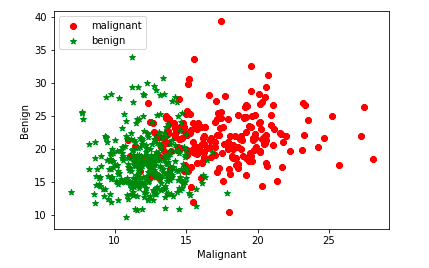
We will use Sklearn Breast Cancer data set to understand SVM RBF kernel concepts in this post. The scatter plot given below represents the fact that the dataset is linearly inseparable and it may be a good idea to apply the kernel method for training the model.

The above plot is created using first two attributes of the sklearn breast cancer dataset as shown in the code sample below:
import pandas as pd
import matplotlib.pyplot as plt
from sklearn import datasets

# Load the breast cancer dataset
#
bc = datasets.load_breast_cancer()
df = pd.DataFrame(data=bc.data)
df["label"] = bc.target

# Scatter plot shown in fig 1
#
plt.scatter(df[0][df["label"] == 0], df[1][df["label"] == 0],
            color='red', marker='o', label='malignant')
plt.scatter(df[0][df["label"] == 1], df[1][df["label"] == 1],
            color='green', marker='*', label='benign')
plt.xlabel('Malignant')
plt.ylabel('Benign')
plt.legend(loc='upper left')
plt.show()
Given that the dataset is non-linear, it is recommended to use kernel method and hence kernel function such as RBF.
SVM RBF Kernel Function Parameters
When using the SVM RBF kernel to train the model, one can use the following parameters:
- Gamma
- C
RBF Kernel Parameter – Gamma Values
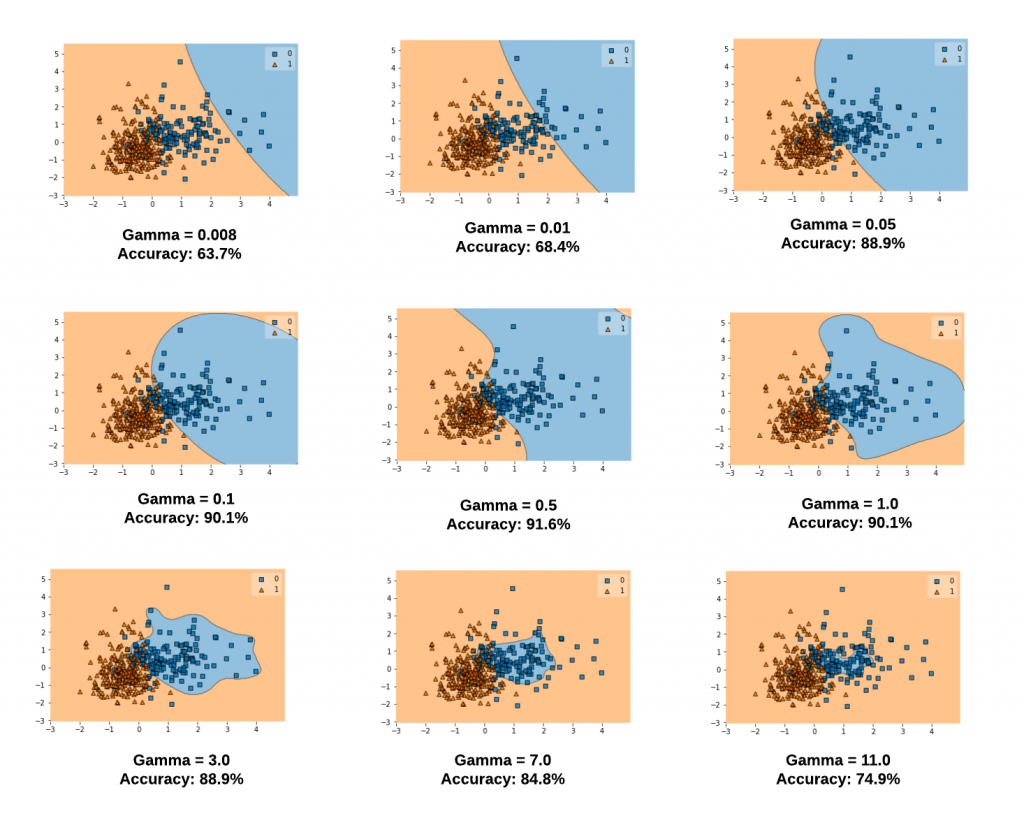
The gamma parameter defines how far the influence of a single training example reaches, with low values meaning ‘far’ and high values meaning ‘close’. The lower values of gamma result in models with lower accuracy and the same as the higher values of gamma. It is the intermediate values of gamma which gives a model with good decision boundaries. The same is shown in the plots given in fig 2.
The plots below represent decision boundaries for different values of gamma with the value of C set as 0.1 for illustration purposes. Note that as the Gamma value increases, the decision boundaries classify the points correctly. However, after a certain point (Gamma = 1.0 and onwards in the diagram below), the model accuracy decreases. It can thus be understood that the selection of appropriate values of Gamma is important. Here is the code which is used.
svm = SVC(kernel='rbf', random_state=1, gamma=0.008, C=0.1)
svm.fit(X_train_std, y_train)

Note some of the following in the above plots:
- When gamma is very small (0.008 or 0.01), the model is too constrained and cannot capture the complexity or “shape” of the data. The region of influence of any selected support vector would include the whole training set. The resulting model will behave similarly to a linear model with a set of hyperplanes that separate the centers of a high density of any pair of two classes. Compare with the diagram in the next section where the decision boundaries for a model trained with a linear kernel is shown.
- For intermediate values of gamma (0.05, 0.1, 0.5), it can see on the second plot that good models can be found.
- For larger values of gamma (3.0, 7.0, 11.0) in the above plot, the radius of the area of influence of the support vectors only includes the support vector itself and no amount of regularization with C will be able to prevent overfitting.
RBF Kernel Parameter – C Values
Simply speaking, the C parameter is a regularization parameter used to set the tolerance of the model to allow the misclassification of data points in order to achieve lower generalization error. Higher the value of C, lesser is the tolerance and what is trained is a maximum-margin classifier. Smaller the value of C, larger is the tolerance of misclassification and what gets trained is a soft-margin classifier that generalizes better than maximum-margin classifier. The C value controls the penalty of misclassification. A large value of C would result in a higher penalty for misclassification and a smaller value of C will result in a smaller penalty of misclassification. With a larger value of C, a smaller margin will be accepted if the decision function is better at classifying all training points correctly. The model may overfit with the training dataset. A lower C will encourage a larger margin, therefore a simpler decision function, at the cost of training accuracy.
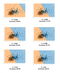
The diagram below represents the decision boundary with different values of C for a model trained with a linear kernel and Sklearn Breast Cancer dataset. Take note of the decision boundary for different values of C. Note that as the value of C increases, the model accuracy increases. This goes in line what we learnt earlier that a smaller value of C allows for greater misclassification and hence the model accuracy will be lower. However, after a certain point (C=1.0), the accuracy ceases to increase.

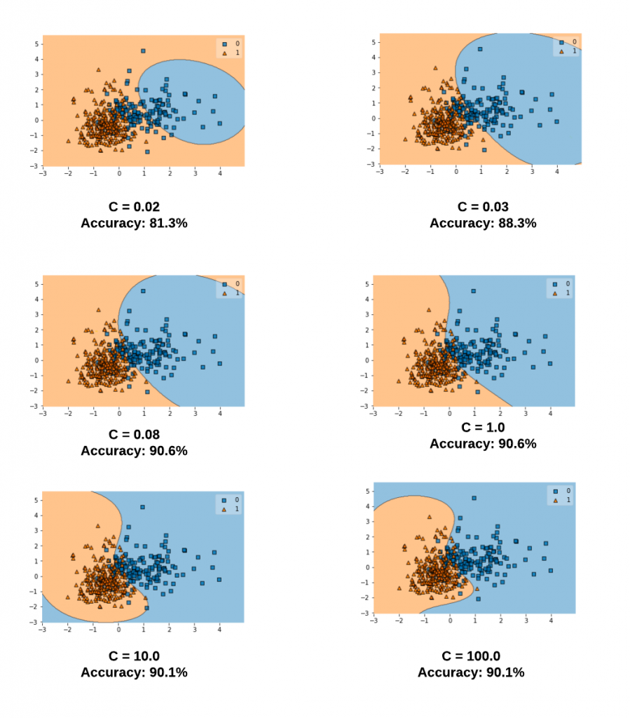
Let’s take a look at different values of C and the related decision boundaries when the SVM model gets trained using RBF kernel (kernel = “rbf”). The diagram below represents the model trained with the following code for different values of C. Note the value of gamma is set to 0.1 and the kernel = ‘rbf’.
svm = SVC(kernel='rbf', random_state=1, gamma=0.1, C=0.02)
svm.fit(X_train_std, y_train)

Tuning RBF Kernel Parameters
Tuning the parameters of an SVM model using the RBF kernel is crucial for achieving good performance. There are different methods for tuning these parameters, including grid search and random search.
Grid search involves defining a grid of possible values for gamma and C and evaluating the model performance for each combination of parameter values. The optimal parameter values are then selected based on the performance metric, such as accuracy or mean squared error, on a holdout set or using cross-validation.
Random search is an alternative approach where the parameter values are randomly sampled from a specified range of values. This method can be more efficient than grid search when the parameter space is large, as it does not require evaluating the model for all possible combinations of parameter values.
Both grid search and random search can be implemented using cross-validation to evaluate the model performance. Cross-validation involves splitting the data into training and validation sets and evaluating the model on the validation set. This process is repeated multiple times using different splits of the data, and the average performance is used to estimate the model performance.
When tuning the parameters of an SVM model using the RBF kernel, it’s important to use an appropriate range of parameter values. The gamma value should typically be varied over a range of values that includes both small and large values, while the C value should be varied over a range of values that includes both small and large values as well.
The following is the Python code representing tuning of Gamma and C values using grid search.
from sklearn.datasets import load_breast_cancer
from sklearn.model_selection import GridSearchCV, train_test_split
from sklearn.svm import SVC
from sklearn.metrics import accuracy_score

# Load breast cancer data
data = load_breast_cancer()
X, y = data.data, data.target

# Split data into training and validation sets
X_train, X_val, y_train, y_val = train_test_split(X, y, test_size=0.3, random_state=42)

# Define grid of parameter values for Gamma and C Parameters
param_grid = {'gamma': [0.1, 0.5, 1.0], 'C': [1, 5, 10]}

# Define SVM model with RBF kernel
svm = SVC(kernel='rbf')

# Perform grid search with cross-validation
grid_search = GridSearchCV(svm, param_grid, cv=5)
grid_search.fit(X_train, y_train)

# Print best parameter values and accuracy on validation set
print("Best gamma value: ", grid_search.best_params_['gamma'])
print("Best C value: ", grid_search.best_params_['C'])
y_pred = grid_search.predict(X_val)
accuracy = accuracy_score(y_val, y_pred)
print("Validation accuracy: ", accuracy)
References
Here are some other posts on similar topics:
- Machine Learning – SVM Kernel Trick Example
- SVM – Understanding C Value with Code Examples
- SVM as Soft Margin Classifier and C Value
- SVM Algorithm as Maximum Margin Classifier
- Sklearn SVM Classifier using LibSVM – Code Example
Conclusion
Here are some of the key points that is covered in this post.
- Gamma and C values are key hyperparameters that can be used to train the most optimal SVM model using RBF kernel.
- The gamma parameter defines how far the influence of a single training example reaches, with low values meaning ‘far’ and high values meaning ‘close’
- Higher value of gamma will mean that radius of influence is limited to only support vectors. This would essentially mean that the model tries and overfit. The model accuracy lowers with the increasing value of gamma.
- The lower value of gamma will mean that the data points have very high radius of influence. This would also result in model having lower accuracy.
- It is the intermediate value of gamma which results in a model with optimal accuracy.
- The C parameter determines how tolerant is the model towards misclassification.
- Higher value of C will result in model which has very high accuracy but which may fail to generalize.
- The lower value of C will result in a model with very low accuracy.
- Large Language Models (LLMs): Four Critical Modeling Stages - August 4, 2025
- Agentic Workflow Design Patterns Explained with Examples - August 3, 2025
- What is Data Strategy? - August 2, 2025
I found it very helpful. However the differences are not too understandable for me