In this post, we will understand the concepts related to SVM (Support Vector Machine) algorithm which is one of the popular machine learning algorithm. SVM algorithm is used for solving classification problems in machine learning.
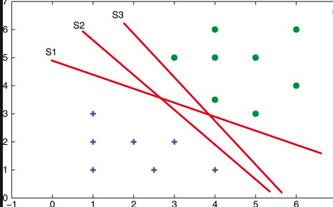
Lets take a 2-dimensional problem space where a point can be classified as one or the other class based on the value of the two dimensions (independent variables, say) X1 and X2. The objective is to find the most optimal line (hyperplane in case of 3 or more dimensions) which could correctly classify the points with most accuracy. In the diagram below, you could find multiple such lines possible.

In the above diagram, the objective is to find the most optimal line / hyperplane which separates the points correctly thereby each point correctly representing the class it belongs to. This problem can be solved using two different algorithms. One of them is Perceptron and another is SVM.
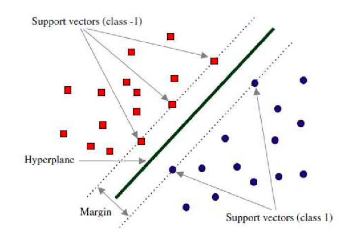
Using the perceptron algorithm, the objective is to find the line/hyperplane which minimise misclassification errors. However, in case of SVMs, the optimisation objective is to maximize the margin such that the points can be classified correctly. The margin is the perpendicular distance from this line/hyperplane to the closest points on either side representing different classes.

In the above diagram, the green line represents the most optimal hyperplane. The red points (Class -1) and blue points (Class 1) represents the points which are closest to the hyperplane (green line). These points are called as support vectors. Due to the fact that the optimisation objective is to find the optimal hyperplane with maximum margin from closest support vectors, SVM models are also called as maximum margin classifier.
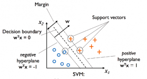
Let’s try and understand the objective function which can be used for optimisation. Take a look at the diagram below.

In the above line, the dashed line represents the most optimal hyperplane or decision boundary. All the points on this hyperplane / line must satisfies the following equation:
[latex]
W^TX = 0
[/latex]
On both the sides of decision boundary lies two other lines which touches the closest point representing two different classes on either sides.
On one side, the line/hyperplane touching the blue circle satisfies the following equation
[latex]
W_0 + W^TX_{neg} = -1
[/latex]
On another side, the line/hyperplane touching the red plus (+) satisfies the following equation:
[latex]
W_0 + W^TX_{pos} = 1
[/latex]
Combining both of the above equations, we get the following equation:
[latex]
W^T(X_{pos} – X_{neg}) = 2
[/latex]
The above equation can be normalized by dividing both the sides with the length of the vector which is the following:
[latex]
\lVert w \rVert = \sqrt{\sum_{j=1}^{m} {w^2}_j}
[/latex]
This is how the equation will look like after dividing both sides with length vector:
[latex]
\frac{W^T(X_{pos} – X_{neg})}{\lVert w \rVert} = \frac{2}{\lVert w \rVert}
[/latex]
The left hand side of the above equation represents the length of distance / margin between the positive and negative line / hyperplane. The objective is to maximise the margin.
Thus, training SVM – maximum margin classifier – becomes a constrained optimisation problem with objective function to maximise as the following:
[latex]
\frac{2}{\lVert w \rVert}
[/latex]
And, the following as the constraints. The equation given below is first inequality constraint function:
[latex]
W_0 + W^TX_{pos} \geq 1
[/latex]
This is the second inequality constraint function:
[latex]
W_0 + W^TX_{neg} \leq -1
[/latex]
An equivalent objective function can be the following which could be minimized with the above constraints.
[latex]
\frac{(\lVert w \rVert)^2}{2}
[/latex]
The downside of maximum margin classifier is that it is difficult to find the hyperplane which correctly classifies all the points. This is where the concept of soft margin classifier comes into picture. This will be discussed in the follow up article.
One can train an SVM classifier using SVC class which is available as part of sklearn.svm module. Check out the code on this page – Training a SVM classifier.
- Three Approaches to Creating AI Agents: Code Examples - June 27, 2025
- What is Embodied AI? Explained with Examples - May 11, 2025
- Retrieval Augmented Generation (RAG) & LLM: Examples - February 15, 2025
I found it very helpful. However the differences are not too understandable for me