
Support Vector Machines (SVMs) are a powerful and versatile machine learning algorithm that has gained widespread popularity among data scientists in recent years. SVMs are widely used for classification, regression, and outlier detection (one-class SVM), and have proven to be highly effective in solving complex problems in various fields, including computer vision (image classification, object detection, etc.), natural language processing (sentiment analysis, text classification, etc.), and bioinformatics (gene expression analysis, protein classification, disease diagnosis, etc.).
In this post, you will learn about the concepts of Support Vector Machine (SVM) with the help of Python code example for building a machine learning classification model. We will work with Python Sklearn package for building the model. As data scientists, it is important to get a good grasp on SVM algorithm and related aspects.
What is Support Vector Machine (SVM)?
Support vector machine (SVM) is a supervised machine learning algorithm that can be used for both classification and regression tasks. At times, SVM for classification is termed as support vector classification (SVC) and SVM for regression is termed as support vector regression (SVR). In this post, we will learn about SVM classifier.
The main idea behind SVM classifier is to find a hyperplane that maximally separates the data points of different classes. In other words, we are looking for the largest margin between the data points belonging to two classes. The hyperplane is selected such that it maximizes the distance between the hyperplane and the closest data points from each class, which are called support vectors. These points have a direct impact on the position and orientation of the hyperplane. The rationale behind having decision boundaries with large margins is that they tend to have a lower generalization error, whereas models with small margins are more prone to overfitting. Hence, SVM classifier is also termed as maximum margin classifier, meaning that it finds the line or hyperplane that has the largest distance to the nearest training data points (support vectors) of any class. The following picture represents the same.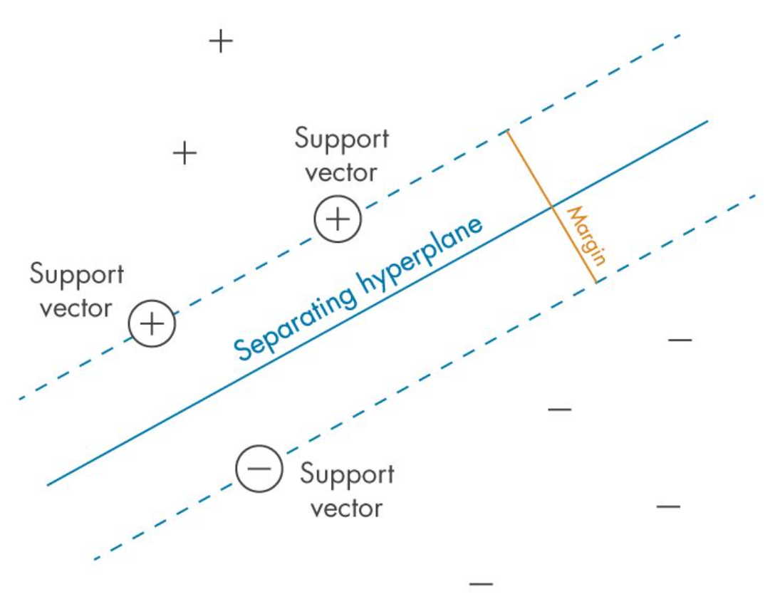
Given labeled training data (for supervised learning), the SVM classification algorithm outputs an optimal hyperplane which categorizes new data examples into different classes. This hyperplane is then used to make predictions on new data points. Let’s take an example to understand Support Vector Machine concepts in a better manner. Say you have been asked to predict whether a customer will churn or not and you have all their past transaction records as well as demographic information. After exploring the data, you’ve found that there’s not much difference between the average transaction amount of customers who churned and those who didn’t. You also found that most of the customers who churned live relatively far from the city center. Based on these findings, you decided to use Support Vector Machine classification algorithm to build your prediction model. Model trained using SVM classification algorithm will be able to classify the customers as high risk (churned) or otherwise.
There are some key concepts that are important to understand when working with SVMs. First, the data points that are closest to the hyperplane are called support vectors. Second, when the data is not linearly separable, SVMs use a technique called kernel trick, which maps the original features into a higher-dimensional feature space where the data is linearly separable. In this new feature space, we can draw a hyperplane that separates the two classes. Third, when working with Python SKlearn SVC algorithm, there are three hyperparameters that results in different SVM models (hypothesis): C, gamma and kernel function.
- C is typically used as a regularization parameter to control overfitting, allowing the algorithm to make more accurate predictions on new data points. The strength of the regularization is inversely proportional to C. C represents the penalty parameter for misclassifying data points. Simply speaking, C controls the trade-off between maximizing the margin and minimizing training error. If C is set too low, the model will fail to accurately classify data points due to underfitting and can produce inaccurate results. A smaller value of C will result in a larger margin, but may lead to more misclassifications. If C is set too high, then the model will have difficulty correctly separating data points due to overfitting and can show poor accuracy scores. A larger value of C will result in a smaller margin, but may lead to better classification accuracy.
The choice of C depends on the problem at hand and the characteristics of the dataset. In general, a smaller value of C is preferred when the dataset is noisy, or when the goal is to have a more generalizable model that can perform well on new, unseen data. A larger value of C is preferred when the dataset is clean and the goal is to maximize classification accuracy on the training data.
As a general guideline, it’s a good idea to start with a smaller value of C and gradually increase it until the desired level of classification accuracy is achieved. However, it’s important to keep in mind that a larger value of C may lead to overfitting, which means that the model performs well on the training data but poorly on new, unseen data. Therefore, it’s important to strike a balance between maximizing the margin and minimizing the classification error, and choose an appropriate value of C based on the specific problem and dataset. - When training a support vector machine (SVM) model using Sklearn SVC algorithm, the gamma hyperparameter can take on two special values: ‘scale’, ‘auto’ or ‘float’. When gamma is set to ‘scale’, it means that the value of gamma is calculated as 1 / (number of features * variance in data). This ensures that all features are given equal importance in the model and produces consistent results no matter how many features are used.
- SVM kernel is a mathematical function that is used to map the data points from one space into another, usually higher dimensional space. When training a support vector machine (SVM) model using Sklearn SVC algorithm, the kernel hyperparameter can take on several values: ‘linear’, ‘poly’, ‘rbf’ and ‘sigmoid’.
- When kernel is set to ‘linear’, it means that the model will use a linear boundary for classification and regression. This is the simplest type of SVM and works best when data are linearly separable.
- When kernel is set to ‘poly’, it means that the model will use polynomial functions of degree higher than 1 for classification. This type of SVM is more suitable for complex non-linear datasets.
- When kernel is set to ‘rbf’, it means that the model will use radial basis funcitons for classification or regression. RBF kernels are capable of dealing with complex multi-class datasets and have good generalization performance with noisy data points.
- When kernel is set to ‘sigmoid’, it means that the model will apply sigmoid functions instead of RBFs for classification or regression tasks. Sigmoid kernels tend to be less sensitive than RBFs with respect to outliers in data but may not generalize as well unless their parameters are tuned properly.
As an example, let’s say we have a dataset with two features (x1 and x2) and two classes (0 and 1). We can visualize this data by plotting it in a two-dimensional space, with each point colored according to its class label. Look at the diagram below.
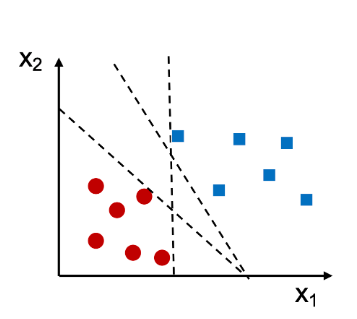
In the above case, we can see that there are different straight lines that can perfectly separate the two classes. However, we can still find a decision boundary that does a pretty good job. This boundary is generated by Support Vector Machine algorithm. Using SVM algorithm, as mentioned above, training the model represents finding the hyperplane (dashed line in the picture below) which separates the data belonging to two different classes by maximum or largest margin. And, the points closest to this hyperplane are called support vectors. Note this in the diagram given below.
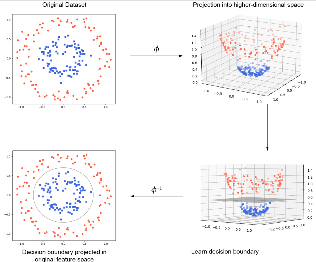
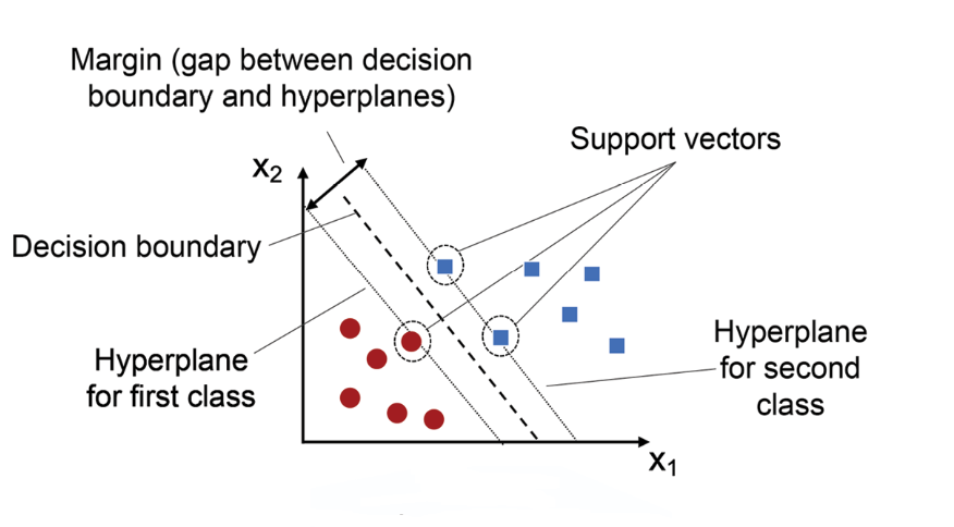 The blue square points represent one class and the red dots represent another class. The black line is the decision boundary learned by an SVM. As you can see, the SVM has placed the boundary in such a way as to maximize the margin between the two classes. Here is a visual representation of how SVM classification works. Note how original data set is projected into higher-dimensional space, then a decision boundary is found and finally the decision boundary is projected into original feature space.
Support vector machines are a powerful tool for classification, but like any machine learning algorithm, they require careful tuning of their hyperparameters in order to achieve optimal performance. The most important hyperparameters are the kernel function and the regularization parameters such as C and gamma. The kernel function determines how data points are transformed into higher dimensional space, and the regularization parameter controls the trade-off between model complexity and overfitting. In addition, the Support Vector Machine also has a number of other important hyperparameters that can be adjusted to improve performance, including the maximum number of iterations, the tolerance for error, and the learning rate. By carefully tuning these hyperparameters, it is possible to achieve significantly better performance from a Support Vector Machine. Here are related post on tuning hyperparameters for building an optimal SVM model for classification:
Support vector machine (SVM) Python example
The following steps will be covered for training the model using SVM while using Python code:
- Load the data
- Create training and test split
- Perform feature scaling
- Instantiate an SVC classifier
- Fit the model
- Measure the model performance
First and foremost we will load appropriate Sklearn modules and classes.
# Basic packages
import numpy as np
import pandas as pd
import matplotlib.pyplot as plt

# Sklearn modules & classes
from sklearn.linear_model import Perceptron, LogisticRegression
from sklearn.svm import SVC
from sklearn.model_selection import train_test_split
from sklearn.preprocessing import StandardScaler
from sklearn import datasets
from sklearn import metrics
Lets get started with loading the data set and creating the training and test split from the data set. Pay attention to the stratification aspect used when creating the training and test split. The train_test_split class of sklearn.model_selection is used for creating training and test split.
# Load the data set; In this example, the breast cancer dataset is loaded.
bc = datasets.load_breast_cancer()
X = bc.data
y = bc.target

# Create training and test split
X_train, X_test, y_train, y_test = train_test_split(X, y, test_size=0.3, random_state=1, stratify=y)
Next step is to perform feature scaling. The reason for doing feature scaling is to make sure that data for different features are in the same range. The StandardScaler class of sklearn.preprocessing is used.
sc = StandardScaler()
sc.fit(X_train)
X_train_std = sc.transform(X_train)
X_test_std = sc.transform(X_test)
Next step is to instantiate a SVC (Support Vector Classifier) and fit the model. The SVC class of sklearn.svm module is used.
# Instantiate the Support Vector Classifier (SVC)
svc = SVC(C=1.0, random_state=1, kernel='linear')

# Fit the model
svc.fit(X_train_std, y_train)
Finally, it is time to measure the model performance. Here is the code for doing the same:
# Make the predictions
y_predict = svc.predict(X_test_std)

# Measure the performance
print("Accuracy score %.3f" %metrics.accuracy_score(y_test, y_predict))
The performance of the model will turn out to be 0.953.
Conclusion
In conclusion, Support Vector Machines (SVMs) are powerful learning models that can be used for both classification and regression tasks. SVMs work by mapping data points into higher dimensional feature space, which allows them to capture nonlinear relationships between features and perform complex classifications and regressions. Python provides several libraries for using SVMs efficiently such as scikit-learn and pySVM, making it easy to get started with SVM implementation in Python. By following the example in this guide, you now know more about what SVMs are capable of, how they work, and how to use them in practice.

Check out my latest book titled as First Principles Thinking: Building winning products using first principles thinking.
- Questions to Ask When Thinking Like a Product Leader - July 3, 2025
- Three Approaches to Creating AI Agents: Code Examples - June 27, 2025
- What is Embodied AI? Explained with Examples - May 11, 2025
So informative and clearly explained with code.
while predicting for an unseen data-point, do we also need to perform standardization of it before feeding it to the model?
Yes, if you have standardized (or normalized) your training data before training your models, you should also standardize any unseen data-points before making predictions. This is because the model has been trained on data with a certain scale and distribution, so it expects inputs with the same scale and distribution when making predictions.