Independent Samples T-test: Formula, Examples, Calculator

Last updated: 21st Dec, 2023

As a data scientist, you may often come across scenarios where you need to compare the means of two independent samples. In such cases, a two independent samples t-test, also known as unpaired two samples t-test, is an essential statistical tool that can help you draw meaningful conclusions from your data. This test allows you to determine whether the difference between the means of two independent samples is statistically significant or due to chance.

In this blog, we will cover the concept of independent samples t-test, its formula, real-world examples of its applications and the Python & Excel example (using scipy.stats.ttest_ind function). We will begin with an overview of what an independent samples t-test is, followed by an explanation of two sample t-test formula and related assumptions. Then, we will explore some examples to help you understand how to apply the test in practice. At the end, you also get a calculator for finding out t-statistics and degrees of freedom for independent samples t-test for equal and unequal variance scenarios. Check out other tools on this page – Machine Learning / Statistical Tools.

What is independent samples or unpaired samples T-test?

The independent samples T-test is defined as statistical hypothesis testing technique in which the samples from two independent groups are compared to determine if the means of the associated populations are significantly different. The t-test compares the means of two groups, such as a control group and a treatment group, to determine if the difference between the groups’ means is statistically significant or due to random chance. For example, lets say that we have two independent groups of marketing professionals having similar qualification and we want to compare their income to determine whether their income is significantly different. 

An independent samples t-test compares the means of two groups. The data are interval for the groups. – Basic and Advanced Statistical Tests

Independent samples t-test is also called unpaired two-samples t-test or just unpaired t-test because the test is performed with only two groups that are independent or unpaired or unrelated. The picture below shows the representation of two independent samples and the aspect of their means. 

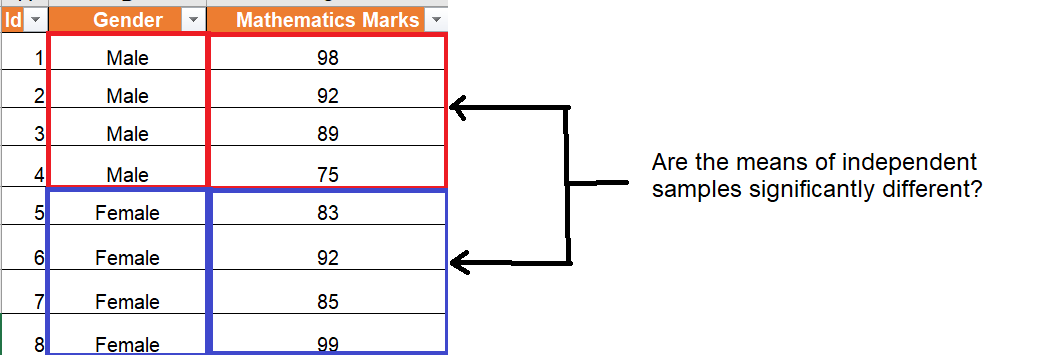
The picture below represents represents the need to compare the means of mathematics marks between two independent group (male and female). Independent samples t-test could be performed.

The 2 samples T-test can also be used for pairwise comparisons when the “two” samples represent the same items tested in different scenarios. The pairwise samples t-test will be dealt with in different blog.

Independent Samples T-Test Examples

Let’s say you want to know if two different brands of batteries have the same average life. You could take a battery from each brand, use them until they die, and record the results. This would be an extremely time-consuming process, and it’s not very likely that you’d get a large enough sample size to draw any conclusions. Another option is to use a independent-samples T-test. This test allows you to compare the averages of two groups without having to measure the batteries’ life spans yourself.

The following are a few real-life examples where independent samples T-test  can be used:

• Business and finance
  • Comparing the sales performance of two products
  • Analyzing the effectiveness of two marketing strategies
• Healthcare and medicine
  • Examining the effects of two treatments on patient outcomes
  • Comparing the mean blood pressure levels of two patient groups
• Social sciences
  • Analyzing the differences in academic performance between two schools
  • Comparing the mean levels of happiness among two age groups

Independent Samples T-test Assumptions

The following are some assumptions related to independent two sample t-test:

• Assumes that the two samples are independent from each other. The samples in no way should be related to each other.
• The size of sample 30 or less is considered as small sample. That said, the size of the sample is not a strict condition for using T-test.
• Assumes that the two populations have normal distributions. This assumption is crucial, especially when the sample size is small. A normal distribution allows us to use the t-distribution, which is the basis of the t-test.
• Assumes the homogeneity of variance between the two groups. The variance of the data in each sample should be equal. If this assumption is violated, it can lead to biased results. The t-test based on this assumption is also called as homoscedastic t-test  If the assumption of equal variances is violated, an alternative version of the t-test, known as Welch’s t-test (or the Welch’s unequal variances t-test), should be used. It’s also called as Heteroscedastic t-test. Welch’s t-test does not assume equal variances and is generally more robust to this kind of violation. It adjusts the degrees of freedom used in the t-test to account for the variance differences, providing a more accurate p-value when variances are unequal.
• Assumes that measurements made on the same group of objects are statistically independent of each other.
• Assumes that all observations within each sample are randomly selected and independently distributed. Random sampling helps to ensure that the sample is representative of the population, reducing the likelihood of sampling bias.
• Assumes that there is an equal or nearly equal sample size between the two groups being tested.

Independent Samples T-Test Formula (Lack of Homogeneity of Variances)

The t-statistics formula for independent samples t-test is different based on whether the variance within the two different groups are same / equal or different (statistically). When the variances of populations are not equal, the two samples t-test formula (equation) for t-statistics is following:

Where X̄1 is mean of first sample, X̄2 is mean of second sample, μ1 is the mean of first population, μ2 is the mean of second population, s1 is the standard deviation of first sample, s2 is the standard deviation of second sample, n1 is the size of the first sample, n2 is the size of the second sample.

The degrees of freedom formula in two-sample t-test can be calculated as the sum of two sample sizes minus two.

Degrees of freedom, df = n1 + n2 – 2

A confidence interval for the difference between two means specifies a range of values within which the difference between the means of the two populations may lie. The difference between the means of two populations can be estimated based on the following formula:

Difference in population means = Difference in sample means +/- T*standard error

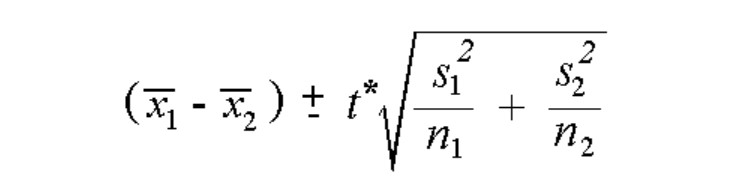
In above formula, the standard error is the square root term.

Independent Two Samples T-test Formula (Equal Population Variances or Standard Deviations)

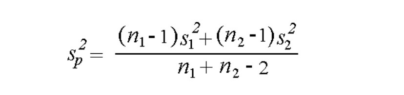
In case, the two populations’ variances or standard deviations are equal, the formula termed as pooled t-statistics is used based on the usage of pooled standard deviations of the two samples. The following is  pooled t-statistics formula for independent samples t-test:

In the above formula, Sp is termed as pooled standard deviation. The formula for pooled variance can be calculated based on the following:

The formula for the degree of freedom in two sample t-test can be calculated as the sum of two sample sizes minus two.

Degrees of freedom, df = n1 + n2 – 2

When independent-samples T-test instead of independent-samples Z-test?

Two independent samples t-test and z-test are both statistical tests used to compare the means of two independent samples. However, the choice between the two tests depends on the characteristics of the data and the assumptions that we can make about the population.

In general, a two independent samples z-test is appropriate when we know the population standard deviation and the sample sizes are large. This is because, when sample sizes are large, the sample means are typically normally distributed, and the z-test assumes normality in the population.

On the other hand, a two samples t-test is more appropriate when we do not know the population standard deviation and the sample sizes are small. This is because, when the sample size is small, the sample means may not be normally distributed, and the t-test can provide a more accurate estimate of the population mean. 

Here is the summary of which tests out of z-test or t-test to use in which scenarios:

Two independent samples z-test:

• Large sample size (typically > 30)
• Known population standard deviation
• Normally distributed population

Two independent samples (unpaired) t-test:

• Small sample size (typically < 30)
• Unknown population standard deviation
• Population may not be normally distributed

Independent Samples T-test: T-Statistics Calculation Example

Lets say we need to compare the performance of two call centers in terms of average call lengths and find out if the difference is statistically significant or the difference is a chance occurrence. To start with, we will need to formulate the null and alternate hypothesis. Note that this will be two-tailed T-test as we are performing null hypothesis based on equality of average call length between two call centers.

Null hypothesis, H0: There is no difference between the average call length between two call centers.

Alternate hypothesis, Ha: There is a difference between the average call length and hence the performance.

We randomly select 20 calls from each call center and calculate the average call lengths. The two call centers seem to have different average call lengths. Is this difference statistically significant?

First, we need to calculate the two sample means and standard deviations:

Call Center A: Sample mean, X̄1 = 122 seconds, SD, S1 = 15 seconds, n1 = 20

Call Center B: Sample mean, X̄2 = 135 seconds, SD, S2 = 20 seconds, n2 = 20

Next, we use a two-sample t-test to determine if the difference between two sample means is statistically significant. We will use a 95% confidence level and α = 0.05.

The two-sample t-statistic is calculated as the following assuming that the standard deviations of the population is not same and the population mean is same.

t = ((135 – 122) – 0)/SQRT((20*20/20) + ((15*15)/20))

t = 13/SQRT(20 + 11.25)

t = 13/SQRT(31.25)

t = 2.3256

The value of degrees of freedom can be calculated as the following:

Degree of freedom, df = n1 + n2 -2 = 20 + 20 – 2 = 38

The critical value of a two-tailed T-test with degrees of freedom as 38 and level of significance as 0.05 comes out to be 2.0244. Since the current t-value of 2.3256 is greater than the critical value of 2.0244, one can reject the null hypothesis that there is no difference between the performance in terms of the call length time. Thus, based on the given evidence, the alternate hypothesis stands as true.

Independent Samples T-test: Python Example

The independent (two) samples T-test output can be used to reject null hypothesis or otherwise in two different ways. They are the following:

• Compare the p-value with the level of significance.
• Compare the t-statistics with critical region

Compare the P-Value with Level of Significance

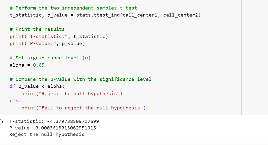
The following represents Python code example for independent samples T-test taking into account the hypothesis discussed in the previous section. The call length observations are, however, different than the previous section. In the code below, the p-value is compared with the level of significance

import numpy as np
from scipy import stats
# Observations for call center 1
call_center1 = [12.5, 11.2, 13.1, 10.8, 11.9, 10.5, 12.4, 12.9, 11.7, 13.2]
# Observations for call center 2
call_center2 = [14.3, 13.1, 15.2, 12.7, 13.9, 13.5, 14.1, 12.8, 13.7, 15.5]
# Perform the two independent samples t-test
t_statistic, p_value = stats.ttest_ind(call_center1, call_center2)
# Print the results
print("T-statistic:", t_statistic)
print("P-value:", p_value)
# Set significance level (α)
alpha = 0.05
# Compare the p-value with the significance level
if p_value < alpha:
    print("Reject the null hypothesis")
else:
    print("Fail to reject the null hypothesis")

The following gets printed as an output. Note that the p-value is less than the level of significance, 0.05, and hence the null hypothesis is rejected.

Note some of the following in above Python code example:

1. The ttest_ind function from the scipy.stats module was used. This function calculates the t-statistic and the p-value.
2. The significance level (α) was set to 0.05, which is a commonly used value.
3. The p-value was compared with the significance level.
4. If the p-value is less than α (0.05), we print “Reject the null hypothesis,” indicating that there is a significant difference in the average call length between the two call centers.
5. If the p-value is greater than or equal to α (0.05), we print “Fail to reject the null hypothesis,” indicating that there is not enough evidence to conclude a significant difference in the average call length between the two call centers.

Compare the T-statistics value with Critical Region Value

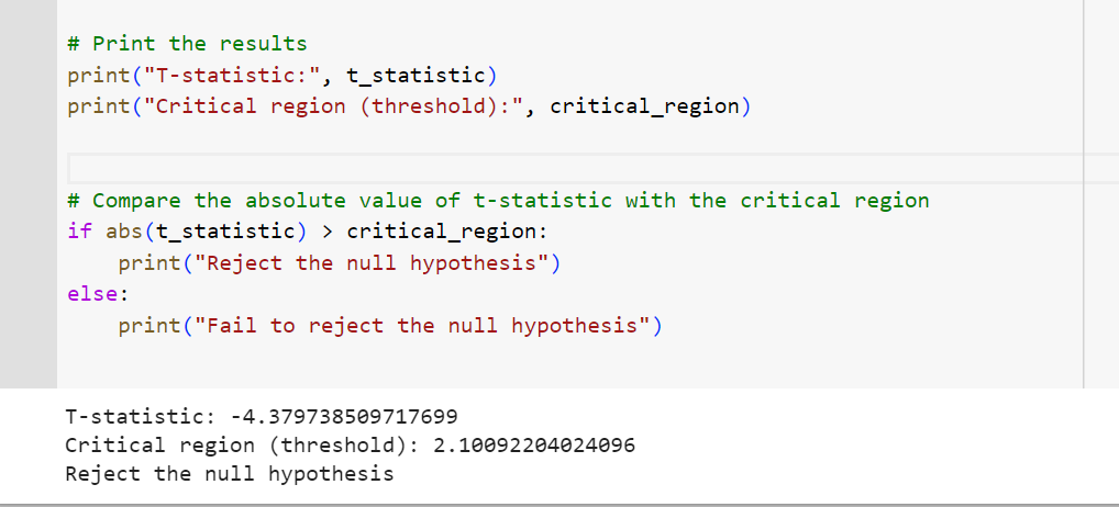
The following Python code represents how the output of independent samples T-test can be used to reject the null hypothesis or otherwise by comparing the value of t-statistics and the critical region (threshold).

import numpy as np
import matplotlib.pyplot as plt
from scipy import stats
# Observations for call center 1
call_center1 = [12.5, 11.2, 13.1, 10.8, 11.9, 10.5, 12.4, 12.9, 11.7, 13.2]
# Observations for call center 2
call_center2 = [14.3, 13.1, 15.2, 12.7, 13.9, 13.5, 14.1, 12.8, 13.7, 15.5]
# Perform the two independent samples t-test
t_statistic, p_value = stats.ttest_ind(call_center1, call_center2)
# Set significance level (α)
alpha = 0.05
# Compute critical region values
df = len(call_center1) + len(call_center2) - 2
critical_region = stats.t.ppf(1 - alpha / 2, df)
# Print the results
print("T-statistic:", t_statistic)
print("Critical region (threshold):", critical_region)
# Compare the absolute value of t-statistic with the critical region
if abs(t_statistic) > critical_region:
    print("Reject the null hypothesis")
else:
    print("Fail to reject the null hypothesis")

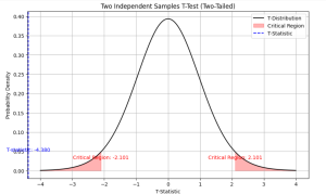
The output shows like the following. Note that the value of t-statistics (-4.3797) is less than the critical region value (negative of 2.1009 = -2.1009 owing to two-tailed t-test) and hence the null hypothesis will be rejected.

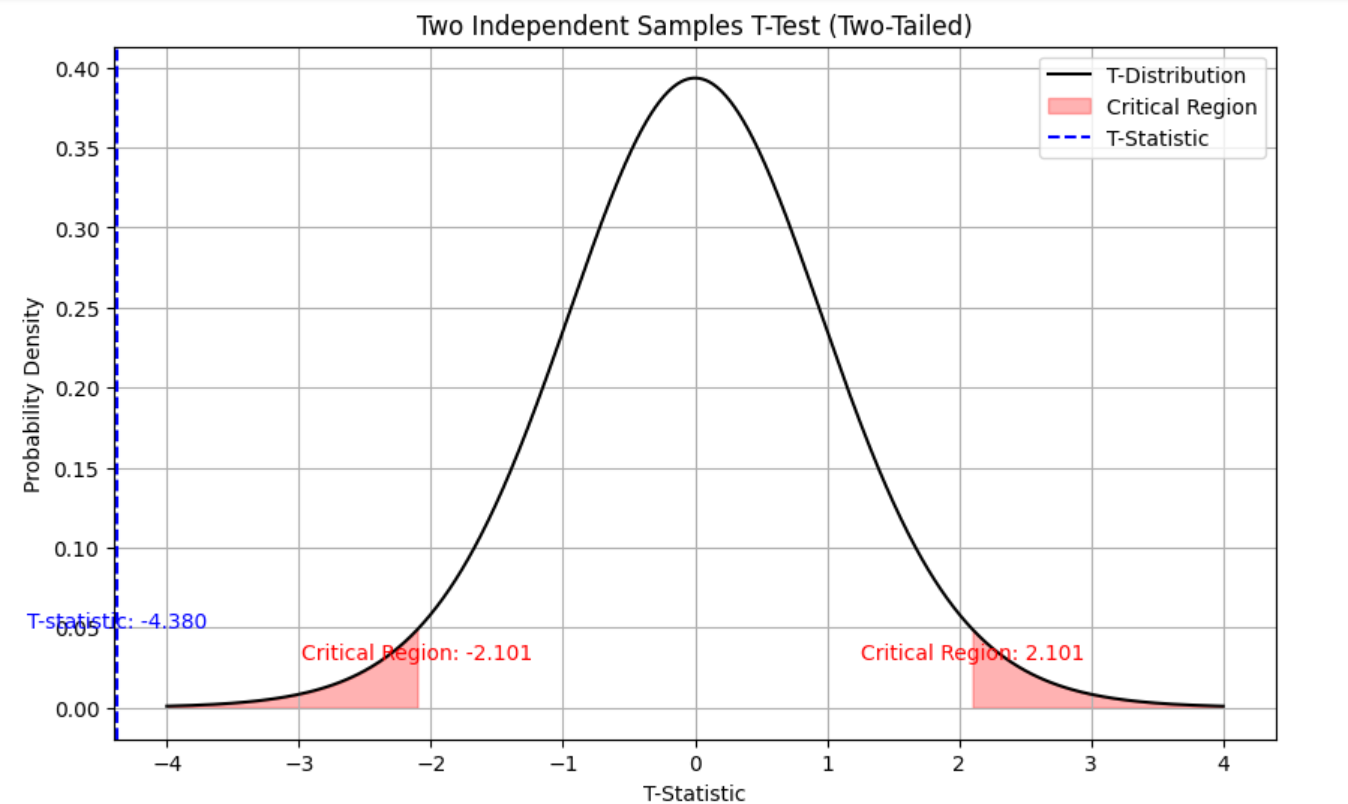
The above can also be understood using the following plot which shows that the value of t-statistics is less than that of the critical region on the negative side and hence, null hypothesis can be rejected,

Independent Samples T-Test using Excel: Example

Performing a two-sample t-test in Excel involves a few key steps. I’ll guide you through these using a real-world example. Let’s consider a scenario where we want to compare the mean scores of two different groups, such as test scores from two different classrooms.

Suppose we have the following data for two classes, Xth A and Xth B for Mathematics:

• Classroom Xth A: A set of test scores.
• Classroom Xth B: Another set of test scores.

We want to determine if there is a statistically significant difference in the average scores between the two classrooms. The following steps can be taken:

1. Collect the Data:
   • Classroom A Scores: e.g., 85, 90, 88, 93, 95
   • Classroom B Scores: e.g., 78, 82, 80, 79, 81
2. Enter the Data in Excel:
   • Open a new Excel worksheet.
   • Enter the scores for Classroom A in one column (say Column A).
   • Enter the scores for Classroom B in the next column (Column B).
3. Label Your Data:
   • It’s good practice to label your columns. You might put “Classroom A” in cell A1 and “Classroom B” in cell B1.
4. Calculate the Mean and Standard Deviation for Each Group (optional but useful):
   • You can use Excel functions to do this. For example, in a new cell, write =AVERAGE(A2:A6) for the mean of Classroom A and =STDEV.S(A2:A6) for the standard deviation. Repeat for Classroom B.
5. Use the T-Test Function:
   • Excel has a built-in function for performing a t-test. You will use the T.TEST function.
   • Syntax: =T.TEST(array1, array2, tails, type)
     • array1 and array2 are the ranges containing your data.
     • tails specifies the number of distribution tails. Use 1 for a one-tailed test and 2 for a two-tailed test.
     • type is the kind of t-test. Use 1 for paired, 2 for two-sample equal variance (homoscedastic), and 3 for two-sample unequal variance (heteroscedastic). For our example, we would typically use 3.
6. Interpreting the Result:
   • The function will return a p-value.
   • If the p-value is less than your significance level (commonly 0.05), you can conclude there is a statistically significant difference between the two sets of scores.
7. Document Your Findings:
   • It’s important to properly document your results and methodology for transparency and reproducibility.

Example Calculation

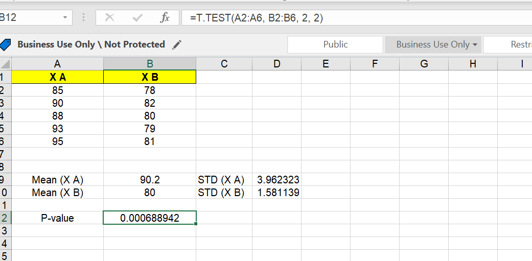
Let’s say your data is in cells A2:A6 for Classroom A and B2:B6 for Classroom B, and you want to perform a two-tailed test assuming unequal variances. We used the value of type as 2 (2 for two-sample equal variance (homoscedastic)). You would enter:

=T.TEST(A2:A6, B2:B6, 2, 2)

The result will be your p-value, which you can use to determine statistical significance.

The following snapshot demonstrates the calculation in an excel spreadsheet.

Frequently Asked Questions (FAQs)

Here are few most commonly asked FAQs related to independent samples t-test:

• How to identify problems where independent samples t-test can be used as a solution?
  • To identify situations where an independent two samples t-test is appropriate, focus on these top three criteria:
    • Two Independent Groups: The core requirement is having two separate, independent groups for comparison. These groups should not overlap or influence each other, such as two different classes of students or patients receiving different treatments.
    • Continuous Dependent Variable: The variable you are comparing between the two groups must be continuous. This means it should represent data that can take on a range of values, like heights, weights, or test scores.
    • Research Question Focused on Comparing Means: The t-test is specifically designed to compare the means (average values) of the two groups. Your research question should aim to find out if there is a significant difference in these means, such as whether one teaching method results in higher test scores than another.
• How do I assess Homogeneity of Variances assumption before applying independent samples t-test?
  • Assessing the homogeneity of variances assumption, an important prerequisite for an independent samples t-test, involves verifying whether the variances in the two groups you are comparing are similar. Here are the common methods to assess this:
    • Levene’s Test: This is the most widely used method for testing the equality of variances. The null hypothesis for Levene’s Test is that the variances are equal across groups. If the test returns a p-value less than the chosen alpha level (commonly 0.05), you reject the null hypothesis, indicating that the variances are significantly different.
    • Visual Inspection (Box Plots, etc.): Before performing statistical tests, it’s often helpful to visually inspect the data. Box plots can be particularly useful for comparing variances between groups. If the sizes of the boxes (which represent the interquartile range) are notably different, this might suggest a difference in variances.
• What is degrees of freedom in two samples or independent samples t test?
  • The degrees of freedom for a two-sample t-test are calculated based on the sample sizes of the two groups. For a two-sample t-test, the formula for degrees of freedom typically used is: df = n1 + n2 – 2, where n1 is the sample size of the first group and n2 is the sample size of the second group.

Independent Samples T-Test Calculator

Calculate the t-statistics and degrees of freedom for independent samples t-test for equal and unequal variances scenarios.

Conclusion

The two samples t-test for independent samples is a statistical method for comparing two different populations. The t-test can be used when the population standard deviations are not known and the sample size is smaller (less than 30). The two sample t-statistic calculation depends on given degrees of freedom, df = n1 + n2 – 2. If the value of two samples t-test for independent samples exceeds critical T at alpha level, then you can reject null hypothesis that there is no difference between two data sets (H0). Otherwise if two sample T-statistics is less than or equal to critical T at alpha level, then one cannot reject H0; this means both values could have come from same distribution in which case any observed difference would be due to chance alone. Different formulas are required to be used for performing t-test for two independent samples based on whether the variances of two populations are equal or otherwise.

• Author
• Recent Posts

Ajitesh Kumar

I have been recently working in the area of Data analytics including Data Science and Machine Learning / Deep Learning. I am also passionate about different technologies including programming languages such as Java/JEE, Javascript, Python, R, Julia, etc, and technologies such as Blockchain, mobile computing, cloud-native technologies, application security, cloud computing platforms, big data, etc. I would love to connect with you on Linkedin.
Check out my latest book titled as First Principles Thinking: Building winning products using first principles thinking.

Latest posts by Ajitesh Kumar (see all)

• Agentic Reasoning Design Patterns in AI: Examples - October 18, 2024
• LLMs for Adaptive Learning & Personalized Education - October 8, 2024
• Sparse Mixture of Experts (MoE) Models: Examples - October 6, 2024