In this post, you will learn about the concepts of Tensor Broadcasting with the help of Python Numpy examples. Recall that Tensor is defined as the container of data (primarily numerical) most fundamental data structure used in Keras and Tensorflow. You may want to check out a related article on Tensor – Tensor explained with Python Numpy examples.
Broadcasting of tensor is borrowed from Numpy broadcasting. Broadcasting is a technique used for performing arithmetic operations between Numpy arrays / Tensors having different shapes. In this technique, the following is done:
- As a first step, expand one or both arrays by copying elements appropriately so that after this transformation, the two tensors have the same shape. If the arrays or tensors are of size 3 x 1 and 1 x 3, then the resulting tensor will have a 3 x 3 shape. For this to happen, the array or tensor with the shape of 3 x 1 will be transformed to 3 x 3 by copying the elements in the first column to two additional columns. Similarly, the tensor with the shape of 1 x 3 will be transformed to tensor 3 x 3 by copying the first row to two additional rows.
- Once the tensor shape transformation happened, carry out the element-wise operations on the resulting arrays.
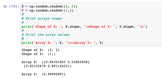
Take a look at the following example where there are two Numpy arrays, X and Y having shapes as (2, 2) and (1, ) respectively. Let’s perform the operation to add X and Y and understand the broadcasting concept in detailed manner. Here is the code representing X & Y created using np.random.random
X = np.random.random((2, 2))
Y = np.random.random((1,))
#
# Print arrays shape
#
print('Shape of X: ', X.shape, '\nShape of Y: ', Y.shape, '\n')
#
# Print the array values
#
print('Array X: ', X, '\n\nArray Y: ', Y)
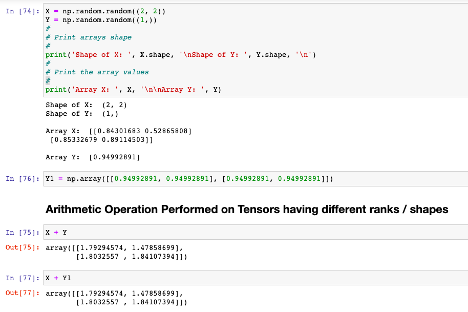
Here is the output of X & Y including their shapes. You may note that the shape of X is (2, 2) – 2D Tensor and Y is (1, ) – 1D Tensor. We will try and perform arithmetic operations on 2D Tensor and 1D Tensor. They have different ranks and shapes. This is where Tensor Broadcasting would come into picture where the Tensors / Numpy arrays will be transformed into compatible shapes to perform the arithmetic operations.

In order to bring the Tensors / Numpy Arrays into compatible shape, this is what is done (as part of the broadcasting process):
- New axes (can be termed as broadcast axes) are added to the smaller tensor to match the ndim of the larger tensor. In the example above, ndim of larger array / Tensor (X) is 2 and ndim of smaller tensor (Y) is 1. New axes will need to be added to Y (1D Tensor).
- The smaller tensor is repeated alongside these new axes to match the full shape of the larger tensor (X – 2D tensor).
Based on above, Y will be internally transformed to the following before arithmetic operation is performed:
Y1 = np.array([[0.94992891, 0.94992891], [0.94992891, 0.94992891]])
Lets validate this by performing arithmetic operation X + Y and X + Y1. You may find that both X + Y and X + Y1 ends up giving same result.

Conclusions
Here is the summary of what you learned about the Tensor broadcasting:
- Tensor broadcasting concept is borrowed from Numpy broadcasting.
- Tensor broadcasting is about bringing the tensors of different dimensions/shape to the compatible shape such that arithmetic operations can be performed on them.
- In broadcasting, the smaller array is found, the new axes are added as per the larger array, and data is added appropriately to the transformed array.
- Mathematics Topics for Machine Learning Beginners - July 6, 2025
- Questions to Ask When Thinking Like a Product Leader - July 3, 2025
- Three Approaches to Creating AI Agents: Code Examples - June 27, 2025
I found it very helpful. However the differences are not too understandable for me