Have you ever felt overwhelmed by all the statistics terminology out there? From sampling distribution to central limit theorem to null hypothesis to p-values to standard deviation, it can be hard to keep up with all the statistical concepts and how they fit into your research. That’s why we created a Statistics Terminologies Cheat Sheet & Examples – a comprehensive guide to help you better understand the essential terms and their use in data analysis. Our cheat sheet covers topics like descriptive statistics, probability, hypothesis testing, and more. And each definition is accompanied by an example to help illuminate the concept even further.
Understanding statistics terminology is critical for data scientists, especially when conducting research and interpreting results. By having a clear understanding of the key statistical concepts and their associated terms, you can better grasp the implications of the data and make informed decisions on how to use it. In addition, having a comprehensive knowledge of statistics terminology also allows you to communicate effectively with other professionals in the field.
So if you’re looking for a handy reference, look no further than our Collection of Statistics Terminologies Cheat Sheet & Examples! Here it goes!
- Statistics: Statistics is the study of data collection, organization, analysis, and interpretation. It is an important tool for understanding relationships between variables and to predict future outcomes. Statistical studies use both samples (a subset of a population) and populations (the entire group) in order to identify patterns and measure relationships. Samples are used to draw inferences about the population as a whole; accuracy depends on how well the sample represents the population and how random the samples are.
- Descriptive statistics: Descriptive statistics represent the numbers which summarizes the data, such as its central tendency (mean, median, mode) or variability / standard deviation (spread). For example, if you wanted to determine the average height of students in a class, you could use descriptive statistics to group them into ranges and then calculate their mean. In this case, mean is an example of a descriptive statistic. In simple words, descriptive statistics represent oversimplification of data to summarize the main content in form of few measures.
- Inferential statistics: Inferential statistics is a branch of statistics that uses data obtained from a sample to make inferences and generalizations about a larger population. This involves taking the insights learned from the sample and using them to make general conclusions about what can be expected in the larger population. For example, suppose you are interested in understanding how much time university students spend studying for their classes each week. To answer this question, you decide to survey 100 students at your university and ask them how many hours per week they spend studying. After analyzing the responses, you may conclude that on average, university students spend approximately 10 hours per week studying for their classes. This conclusion can then be used to infer that this is likely also true of all other university students across the country – not just those surveyed.
- Sample: A sample is a subset of a population used in statistical studies in order to draw inferences about the population as a whole. Samples need to be representative of the entire population; Samples also need to be random in order to be effective for analysis.
- Population: Population in the context of statistics is the entire group that is being studied. It is used as a reference point to understand the sample and draw inferences about the entire group.
- Test statistics: Test statistics are statistical values that measure the degree of association between two variables and the strength of the evidence in a hypothesis test. Test statistics are used to determine the outcome of hypothesis testing. It indicates if a null hypothesis can be rejected or otherwise, based on the data collected from a sample.
- Sample statistics: Sample statistics are metrics calculated from a sample dataset derived from larger population. These values can be used to estimate population parameters, such as mean, variance, and correlations. Sample statistics may also be used in hypothesis tests to determine if a null hypothesis can be rejected or not.
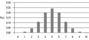
- Data distribution: Data distribution can be defined as a set of all possible outcomes or values of a random variable along with its probability. Data distribution can be used to determine the probability of a certain value occurring in a set. Data distribution can be represented using plot or a graph that shows how the values in a data set are spread out. It can tell us all possible values we’re likely to see in this data set, and how often (frequency of occurrence of each of the values). For example, if most of the values in a data set are clustered around the average, it’s said to have a normal or bell-curve distribution. This means that some values will be higher and some will be lower than the average, but most will be close to it. On the other hand, if the data set has lots of outliers (values much higher or lower than the average), then its distribution is said to be skewed. Data distributions can be either continuous or discrete, and are typically represented graphically with histograms. There are several types of data distributions such as normal, binomial, Poisson, uniform, and exponential distributions.
- Sampling distribution: A sampling distribution is the distribution of a sample statistic (such as the mean) for all possible samples of size n. For example, if a population (frame) contains 500 items, the sampling distribution of the mean for samples of 25 items would be developed by taking every different sample of 25 items from the population of 500 items, computing the mean, then arranging all the sample means in a distribution.
- Sample statistics: Sample statistics is used to represent the descriptive statistics of the sample including its mean, standard deviation, etc. Sample statistics can be used to conclude about the population parameter (such as mean, proportion, etc) with certain confidence intervals. For example, if the mean of the sample (sample statistics) comes out to be [latex]\bar{x}[/latex], it can be used to represent population mean with some confidence interval, such as [latex]\bar{X} = \bar{x} +/- ConfLevel*StdError[/latex] where ConfLevel is confidence interval and StdError is the standard error.
- Standard error: The standard error is a measure of the variability of a sample statistic calculated for the sampling distribution. It is used to estimate how far the sample statistic deviates from the population parameter (such as mean, proportion, etc.). In other words, it helps us determine if any conclusions drawn from our experiment or survey are statistically significant or not. The standard error of a statistic (such as mean) is basically equal to the standard deviation of the population divided by the square root of n (the sample size). Note that as the sample size increases, the standard error decreases and thus overall margin or error decreases. That seems to align well with the intuition. If the population standard deviation is unknown, the sample standard deviation is used.
- Margin of error: The margin of error can be defined, mathematically, as the product of z-value or t-value (determined based on confidence level) and the standard error. Whether to use z-value or t-value depends upon whether population standard deviation is known or size of the sample. If the population standard deviation is known and size of sample is large (more than 30), z-value can be used. If the population standard deviation is unknown or size of the sample is small (less than 30), t-value is used. Conceptually, the margin of error is used to determine the range in which population parameter (such as mean) might fall when we use sample statistics (mean or proportion) to arrive at the population parameter. For a 95% level of confidence, the margin of error will be 1.96*standardError. The value 1.96 is the z-value or the number of standard deviations at 95% level of confidence. For 99% level of confidence, the value comes out to be 2.58. The z-value represents how far a specific value lies from the sample mean (or proportion).
- Central limit theorem: The Central Limit Theorem states that the distribution of sample means approaches a normal or bell-curve distribution as the sample size increases. This means that even if the population from which samples are taken has an unusual or skewed distribution, the average of many sample means will be normally distributed. In other words, as long as we have enough data, then no matter what the actual population looks like, we can use a normal distribution to make predictions about it.
- Mean: The mean can be defined as the average of a set of numbers. It is calculated by adding all of the values in the set and then dividing by the number of values in the set. For example, if we had 3 numbers: 5, 10 and 15, then their mean would be 10 (5 + 10 + 15 = 30, 30 / 3 = 10).
- Median: The median is the middle value of a set of numbers. To calculate the median, first put the numbers in order from lowest to highest. Then, if there are an odd number of values in the set, the median is the middle number. If there are an even number of values in the set, then add the two middle numbers together and divide by two to get the median.
- Mode: The mode is the most frequently occurring value in a set of numbers. For example, if we had [3, 5, 5, 7, 11], then the mode would be 5 since it occurs the most times.
- Variance: Variance is a measure of how spread out a set of numbers is. It calculates the average of the squared differences from the mean. To calculate the variance, first find the mean of your data set. Then for each value in your dataset, subtract the mean and square it. Finally, take the sum of all these values, divide by one less than the total number of items in your dataset, and take its square root to get the variance. Here is formula for variance for a sample:
variance = sqrt(sum(x - mean)² / (n - 1)) - Standard deviation: Standard deviation is a measure of the dispersion of a set of numbers. It basically tells us how much the values are spread out from their average. To calculate standard deviation, first find the variance of the set using the formula above, then take its square root to get the standard deviation.
Standard Deviation = √Variance - Hypothesis testing: Hypothesis testing is a statistical procedure used to determine whether an assertion or hypothesis about a population is true. It uses data taken from a sample of that population to draw conclusions. A null hypothesis that states there is no difference between the observed data and what we would expect if the null hypothesis were true, must first be formulated. Then, an alternative hypothesis is proposed and tested. After performing the test, we can accept or reject the null hypothesis depending on whether it is statistically significant
H0: There is no difference / relationship between X and Y Ha: There is a difference / relationship between X and Y - Null hypothesis: The null hypothesis is a statement that there is no difference between the observed data and what we would expect if the null hypothesis were true. It is usually denoted as
H0and it forms the basis of many statistical tests. - Alternate hypothesis: The alternative hypothesis is a statement that asserts there is a relationship between two variables or that one variable affects the other. Think of it like this: if you were to flip a coin ten times and get nine heads and one tail, the alternative hypothesis would be that the coin isn’t actually fair
- Level of significance: The level of significance is a numerical measure that indicates the probability of a hypothesis being true. It’s usually expressed as a “p-value”, which stands for the probability value. In simpler terms, it’s the chance that an observed result could occur by chance alone – how likely it is that our data or observation is just due to random chance. Put another way, it tells us if our results were due to random luck or if they were significant enough to be considered real and meaningful. If the p-value is higher than your predetermined level of significance, then your results are not statistically significant and you cannot reject the null hypothesis.
- P-value: P-value is the probability of obtaining the results as unusual or extreme as the observed result given the null hypothesis is true. A low value (lower than alpha) would be ideal scenario for rejecting the null hypothesis. If the null hypothesis is true, a very low value of probability or p-value will be a contradiction and hence, would require null hypothesis to be rejected. It’s usually expressed as a decimal, for example 0.03. This means that there is only a 3% chance that the observed result could occur by chance alone given the null hypothesis is true. In simpler terms, it tells us if our results were due to random luck or if they are statistically significant enough to be considered real and meaningful. If the p-value is higher than your predetermined level of significance (usually 0.05 or less), then your results are not statistically significant and you cannot reject the null hypothesis. If the p-value is less than the level of significance, it means that the results are statistically significant and you can reject the null hypothesis.
- Statistical tests: Statistical tests are used to measure the probability that an observed result is due to chance, rather than a real relationship or cause. The goal of a statistical test is to determine whether the results of a hypothesis test are statistically significant, meaning that they cannot be attributed only to randomness or chance alone. All statistical test would require defining a test statistics that would be used to measure the effect or result or outcome of hypothesis test.
- Type I Error: Type 1 error, also known as a false positive, is when a statistical test wrongly rejects the null hypothesis. This means that the test results indicate a significant difference when in reality there is not one. Type 1 errors are more likely to occur when the significance level is set too low.
- Type II Error: Type 2 error, also known as a false negative, is when a statistical test incorrectly fails to reject the null hypothesis. This means that the test results indicate no difference between two datasets when in reality there is a difference. Type 2 errors are more likely to occur when the significance level is set too high.
- Degrees of freedom: Degrees of freedom are the number of values in a statistical calculation that are free to vary. For example, if you know the mean for a sample of 20 values, and you also know 19 of the values, you also know the 20th value. Only 19 are free to vary. Thus, the degree of freedom is 19. The number of degrees of freedom is an input to many statistical tests. For example, degrees of freedom is the name given to the n – 1 denominator seen in the calculations for variance and standard deviation.
- Analysis of Variance (ANOVA): ANOVA, or Analysis of Variance, is a statistical technique used to compare the means of multiple groups. It determines whether there is a statistically significant difference between the observed means of two or more independent groups. ANOVA analyzes the differences in group means by evaluating the variance within each group and the variance between groups.
- One-way ANOVA: One-way ANOVA is a statistical test that measures the differences between two or more independent groups. This type of test is used to determine if there is a statistically significant difference in the means of those groups, while controlling for other variables. To perform 1-way ANOVA test, an analysis of variance (ANOVA) is conducted on one factor (the dependent variable), with multiple related subgroups (or levels). The results of this test determine whether or not there are statistically significant differences between the groups.
- Probability: Probability is a measure of how likely something is to happen. It’s a number between 0 and 1 that expresses the likelihood that an event will occur—the closer the probability value is to 1, the more likely it is that the event will occur. For example, if you flip a coin, there’s an equal chance (50%) of either heads or tails appearing. This would be expressed as
P(heads) = 0.5orP(tails) = 0.5. Probability can also be expressed as odds which are calculated by taking the likelihood of one outcome and dividing it by the total number of possible outcomes. - Probability distribution: Probability distributions are mathematical functions that tell us the probabilities of certain outcomes in an experiment. Probability distribution is used to represent the data distribution. They help us better understand and predict the behavior of random variables—variables whose values are determined by chance. For example, the probability distribution of a coin flip could be denoted as
P(H) = 0.5, meaning that there’s a 50% chance the outcome will be heads. There are many different types of probability distributions, such as binomial, uniform, normal, exponential and Poisson. Each type describes a different kind of phenomenon and is used to study different types of data.
Knowing the concepts and terminologies of statistics is an important part of understanding the bigger picture when it comes to data analysis. This blog is aimed to be a quick reference for beginners, as well as experienced statisticians looking for a refresher and some handy definitions. With this guide in hand, you’ll have all the information you need to start understanding statistics better and make informed decisions with your data.

Check out my latest book titled as First Principles Thinking: Building winning products using first principles thinking.
- Three Approaches to Creating AI Agents: Code Examples - June 27, 2025
- What is Embodied AI? Explained with Examples - May 11, 2025
- Retrieval Augmented Generation (RAG) & LLM: Examples - February 15, 2025
I found it very helpful. However the differences are not too understandable for me