Last updated: 18th Nov, 2023
Dimensionality reduction is an important technique in data analysis and machine learning that allows us to reduce the number of variables in a dataset while retaining the most important information. By reducing the number of variables, we can simplify the problem, improve computational efficiency, and avoid overfitting.
Two popular dimensionality reduction techniques are Principal Component Analysis (PCA) and Linear Discriminant Analysis (LDA). Both techniques aim to reduce the dimensionality of the dataset, but they differ in their objectives, assumptions, and outputs. But how do they differ, and when should you use one method over the other? As data scientists, it is important to get a good understanding around this concept as it is used in building machine learning models. Keep reading to find out with the help of Python & R code & examples.
In this blog post, we will compare and contrast the differences between PCA and LDA, and provide Python & R code examples that illustrate these differences. We will discuss the implications of these differences for selecting between PCA and LDA in different contexts, and provide practical guidance on how to implement these techniques using Python & d.
How does Principal Component Analysis (PCA) work?
Principal Component Analysis (PCA) is an unsupervised learning technique that aims to maximize the variance of the data along the principal components. The goal is to identify the directions (components) that capture the most variation in the data. In other words, it seeks to find the linear combination of features that captures as much variance as possible. The first component is the one that captures the maximum variance, the second component is orthogonal to the first and captures the remaining variance, and so on. PCA is a useful technique for dimensionality reduction, particularly effective, when your data has linear relationships between features – that is, when you can express one feature as a function of the other(s). In such cases, you can use PCA to compress your data while retaining most of the information content by choosing just the right number of features (components).
The following plot can be used to illustrate the PCA concept with 2 principal components.
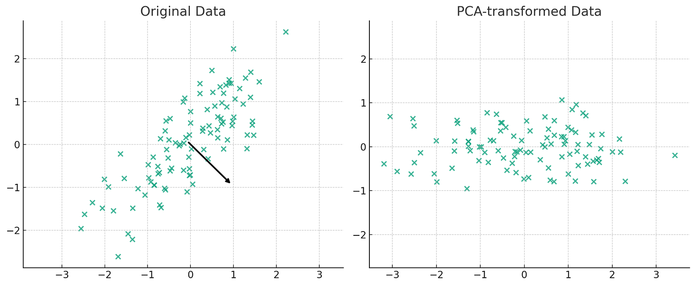
The plot above visually represents the concept of Principal Component Analysis (PCA) with 2 principal components.
-
On the left, you see the original data plotted in its original two-dimensional space. The arrows represent the two principal components found by PCA. These components are the directions in which the data varies the most. The length of the arrows corresponds to the explained variance by each principal component, with longer arrows indicating greater variance.
-
On the right, the data is transformed into the new coordinate system defined by these principal components. This plot shows the data after it has been projected onto the two principal components. The X-axis corresponds to the first principal component, and the Y-axis corresponds to the second principal component.
This visual representation helps to understand how PCA reduces the dimensionality of the data while trying to preserve as much of the data’s variance as possible. In this case, with two principal component, the dimensionality remains the same, but the axes are rotated to align with the directions of maximum variance in the data.
Python Code Example to demonstrate PCA Concepts
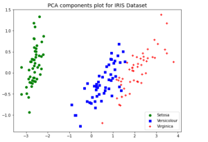
Here’s an Python Sklearn code example to help illustrate how PCA works. We will use IRIS dataset. In the code below, the IRIS dataset is transformed into 2 components and scatter plot is created representing all the three classes such as Setosa, Versicolour and Virginica. Note the usage of sklearn.decomposition.PCA which is a Python’s scikit-learn library, a widely used tool for performing Principal Component Analysis. It offers several parameters that allow users to fine-tune the PCA process according to their specific data and requirements. The most important parameter is n_components that specifies the number of principal components to keep. If not set, all components are kept. It can be an integer or a float between 0 and 1, where in the latter case, it selects the number of components such that the cumulative explained variance ratio is greater than the specified value.
import pandas as pd
import numpy as np
from sklearn.decomposition import PCA
import matplotlib.pyplot as plt
from sklearn import datasets
#
# Load IRIS dataset
#
iris = datasets.load_iris()
#
# Create a dataframe from IRIS dataset
#
df = pd.DataFrame(iris.data, columns=["sepal_length", "sepal_width", "petal_length", "petal_width"])
df["class"] = iris.target
#
# Create PCA transformed dataset with dimensionality
# reduced to 2; n_components = 2
#
pca = PCA(n_components=2)
X_pca = pca.fit(df.iloc[:, 0:4]).transform(df.iloc[:, 0:4])
#
# Create plot from transformed dataset
#
plt.figure(figsize=(8,6))
plt.scatter(X_pca[0:50,0], X_pca[0:50,1], color='green', marker='o', label='Setosa')
plt.scatter(X_pca[50:100,0], X_pca[50:100,1], color='blue', marker='s', label='Versicolour')
plt.scatter(X_pca[100:150,0], X_pca[100:150,1], color='red', marker='+', label='Virginica')
plt.title("PCA components plot for IRIS Dataset", fontsize=14)
plt.legend()
plt.show()

The above plot of data points after PCA was used for dimensionality reduction to 2 components shows a great separation between three different classes. Without the PCA, the plots such as below would represent the fact that classes ain’t separated clearly. This showcases the advantage of why PCA can be used for dimensionality reduction and a model trained with the transformed data will perform better than the original data.
#
# Create plot from original IRIS dataset
#
plt.figure(figsize=(8,6))
plt.scatter(df.iloc[0:50,0], df.iloc[0:50,1], color='green', marker='o', label='Setosa')
plt.scatter(df.iloc[50:100,0], df.iloc[50:100,1], color='blue', marker='s', label='Versicolour')
plt.scatter(df.iloc[100:150,0], df.iloc[100:150,1], color='red', marker='+', label='Virginica')
plt.title("Scatter plot without PCA transformation", fontsize=14)
plt.legend()
plt.show()
R Code Example to demonstrate PCA Concepts
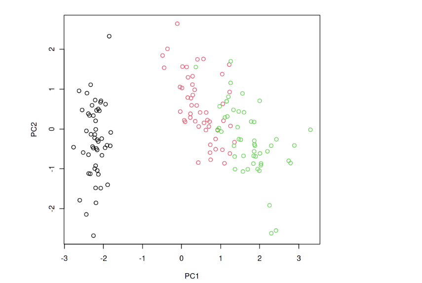
Let’s look at the R code snippets to demonstrate Principal Component Analysis (PCA). This code performs PCA on the famous Iris dataset. It scales the data, computes PCA, and then plots the first two principal components.
# Load required library
library(stats)

# Example dataset
data(iris)
X <- iris[, -5]  # Exclude the species column

# Performing PCA
pca_result <- prcomp(X, scale. = TRUE)

# Summary of PCA
summary(pca_result)

# Plotting PCA
plot(pca_result$x[,1:2], col = iris$Species)
The following plot gets printed.
How does Linear Discriminant Analysis (LDA) work?
Linear discriminant analysis (LDA) is another linear transformation technique that is used for dimensionality reduction. Unlike PCA, however, LDA is a supervised learning method, which means it takes class labels into account when finding directions of maximum variance. LDA aims to maximize the separation between different classes in the data. The goal is to identify the directions that capture the most separation between the classes. This makes LDA particularly well-suited for classification tasks where you want to maximize class separability.
Python Code Example to demonstrate LDA concepts
As with PCA, LDA assumes that your data is centered around the origin and that your features are uncorrelated with one another. You can center and decorrelate your data using scikit-learn’s StandardScaler and LinearDiscriminantAnalysis classes, respectively. Once your data has been cleaned and transformed, you can fit an LDA model to it using scikit-learn’s fit_transform() method. This will return a projected version of your data that has been reduced to the desired number of dimensions while maximizing class separability. In the code below, the IRIS dataset is transformed into 2 components and scatter plot is created representing all the three classes such as Setosa, Versicolour and Virginica.
Note the usage of sklearn.discriminant_analysis.LinearDiscriminantAnalysis that represents a classifier that establishes a linear decision boundary.
import pandas as pd
import numpy as np
from sklearn.discriminant_analysis import LinearDiscriminantAnalysis
import matplotlib.pyplot as plt
from sklearn import datasets
#
# Load IRIS dataset
#
iris = datasets.load_iris()
#
# Create a dataframe from IRIS dataset
#
df = pd.DataFrame(iris.data, columns=["sepal_length", "sepal_width", "petal_length", "petal_width"])
df["class"] = iris.target
#
# Create LDA transformed dataset with dimensionality
# reduced to 2; n_components = 2
#
lda = LinearDiscriminantAnalysis(n_components=2)
X_lda = lda.fit(df.iloc[:, 0:4], df.iloc[:, -1]).transform(df.iloc[:, 0:4])
#
# Create plot from transformed dataset
#
plt.figure(figsize=(8,6))
plt.scatter(X_lda[0:50,0], X_lda[0:50,1], color='green', marker='o', label='Setosa')
plt.scatter(X_lda[50:100,0], X_lda[50:100,1], color='blue', marker='s', label='Versicolour')
plt.scatter(X_lda[100:150,0], X_lda[100:150,1], color='red', marker='+', label='Virginica')
plt.title("LDA components plot for IRIS Dataset", fontsize=14)
plt.legend()
plt.show()
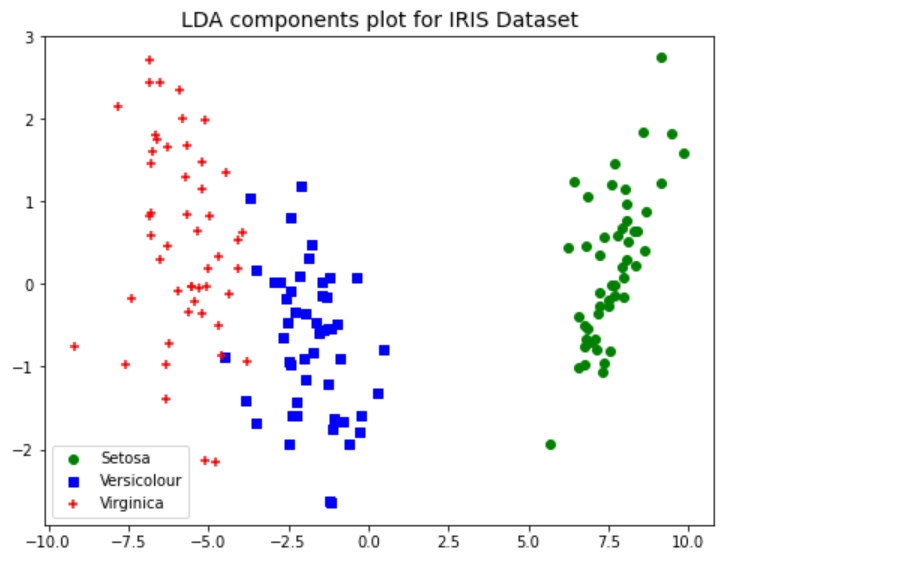
As like PCA transformation, LDA transformation also results in clear separation of IRIS dataset classes which would not have been possible with scatter plot on original dataset.
R Code Example to demonstrate LDA concepts
Let’s use a different dataset for the LDA example. A good alternative is the mtcars dataset, which is also built into R. This dataset comprises various attributes of cars. For demonstration purposes, we’ll classify cars based on their transmission type (automatic or manual), represented by the am column in the dataset (0 = automatic, 1 = manual). It aims to find a linear combination of features that best separates the two transmission types. Remember, LDA is most effective when the response variable is categorical.
Here’s how you can apply LDA to the mtcars dataset:
library(MASS)  # Load MASS package for LDA

# Using the mtcars dataset
data(mtcars)

# Convert transmission type to a factor for classification
mtcars$am <- as.factor(mtcars$am)

# Perform LDA with transmission type as the response variable
lda_result <- lda(am ~ ., data = mtcars)

# Print summary of LDA
print(lda_result)

# You can plot the LDA results
plot(lda_result, col = as.integer(mtcars$am))
PCA vs LDA: Key Differences
Here are some key differences between PCA and LDA:
- Objective: PCA is an unsupervised technique that aims to maximize the variance of the data along the principal components. The goal is to identify the directions that capture the most variation in the data. LDA, on the other hand, is a supervised technique that aims to maximize the separation between different classes in the data. The goal is to identify the directions that capture the most separation between the classes.
- Supervision: PCA does not require any knowledge of the class labels of the data, while LDA requires labeled data in order to learn the separation between the classes.
- Dimensionality Reduction: PCA reduces the dimensionality of the data by projecting it onto a lower-dimensional space, while LDA reduces the dimensionality of the data by creating a linear combination of the features that maximizes the separation between the classes.
- Output: PCA outputs principal components, which are linear combinations of the original features. These principal components are orthogonal to each other and capture the most variation in the data. LDA outputs discriminant functions, which are linear combinations of the original features that maximize the separation between the classes.
- Interpretation: PCA is often used for exploratory data analysis, as the principal components can be used to visualize the data and identify patterns. LDA is often used for classification tasks, as the discriminant functions can be used to separate the classes.
- Performance: PCA is generally faster and more computationally efficient than LDA, as it does not require labeled data. However, LDA may be more effective at capturing the most important information in the data when class labels are available.
LDA vs PCA: When to use which method?
PCA is an unsupervised learning algorithm while LDA is a supervised learning algorithm. This means that PCA finds directions of maximum variance regardless of class labels while LDA finds directions of maximum class separability.
So now that you know how each method works, when should you use PCA vs LDA for dimensionality reduction? In general, you should use LDA when your goal is classification – that is, when you have labels for your data points and want to predict which label new points will have based on their feature values . On the other hand, if you don’t have labels for your data or if your goal is simply to find patterns in your data (not classification), then PCA will likely work better .
That said, there are some situations where LDA may outperform PCA even when you’re not doing classification . For example , imagine that your data has 100 features but only 10% of those features are actually informative (the rest are noise). If you run PCA on this dataset, it will identify all 100 components since its goal is simply to maximize variance . However , because only 10% of those components are actually informative, 90% of them will be useless. If you were to run LDA on this same dataset, it would only identify 10 components since its goal capturing class separability would be better served by discarding noisy features. Thus, if noise dominates your dataset then LDA may give better results even if your goal isn’t classification! Because LDA makes stronger assumptions about the structure of your data, it will often perform better than PCA when your dataset satisfies those assumptions but worse when it doesn’t.
Conclusion
So which technique should you use? That depends on what kind of data you’re working with and what your goals are. If you’re working with labeled data and your goal is to find a low-dimensional representation that maximizes class separability, then LDA is probably your best bet. However, if your goal is simply to find a low-dimensional representation that retains as much information as possible or if you’re working with unlabeled data, then PCA might be a better choice.
In general, it’s always worth trying both techniques on your dataset and seeing which one gives you the best results!

Check out my latest book titled as First Principles Thinking: Building winning products using first principles thinking.
- Questions to Ask When Thinking Like a Product Leader - July 3, 2025
- Three Approaches to Creating AI Agents: Code Examples - June 27, 2025
- What is Embodied AI? Explained with Examples - May 11, 2025
I found it very helpful. However the differences are not too understandable for me