Machine Learning – Sensitivity vs Specificity Differences, Examples

Last updated: 18th Nov, 2023

Machine learning (ML) models are increasingly being used to learn from data and make decisions or predictions based on that learning. When it comes to evaluating the performance of these ML models, there are several important metrics to consider. One of the most important metrics is the accuracy of the model, which is typically measured using sensitivity and specificity. Sensitivity and specificity are two important concepts often used in the context of classification tasks in machine learning. They help to evaluate the performance of a classification model. 

In this post, we will try and understand the concepts behind machine learning model evaluation metrics such as sensitivity and specificity with the help of real-world Python code examples. The post also describes the differences between sensitivity and specificity. You may want to check out another related post titled ROC Curve & AUC Explained with Python examples.

Sensitivity explained with Real-life Examples

Sensitivity is a measure of how well a machine learning model can detect positive instances. It is also known as the true positive rate (TPR) or recall. In other words, sensitivity measures the proportion of actual positives that are correctly identified as such (e.g., the percentage of sick people who are correctly identified as having the condition). Sensitivity is used to evaluate model performance because it allows us to see how many positive instances the model was able to correctly identify. Let’s consider an example of a medical test for a rare disease to understand the concept of sensitivity. Suppose that the test has a sensitivity of 95%. This means that if 100 people who have the disease take the test, the test will correctly identify 95 of them as positive, but it will miss 5 of them (false negatives).

As shown above, A model with high sensitivity will have few false negatives, which means that it is missing a few of the positive instances. In various use cases, it is important for the models to have high sensitivity because we want our models to be able to find all of the positive instances in order to make accurate predictions. The sum of sensitivity (true positive rate) and false negative rate would be 1. The higher the true positive rate, the better the model is in identifying the positive cases in the correct manner.

Mathematically, sensitivity or true positive rate can be calculated as the following:

Sensitivity = (True Positive)/(True Positive + False Negative)

A high sensitivity means that the model is correctly identifying most of the positive results, while a low sensitivity means that the model is missing a lot of positive results.

The following are the details in relation to True Positive and False Negative used in the above equation.

• True Positive: Persons predicted as suffering from the disease (or unhealthy) are actually suffering from the disease (unhealthy); In other words, the true positive represents the number of persons who are unhealthy and are predicted as unhealthy.

• False Negative: Persons who are actually suffering from the disease (or unhealthy) are actually predicted to be not suffering from the disease (healthy). In other words, the false-negative represents the number of persons who are unhealthy and got predicted as healthy. Ideally, we would seek the model to have low false negatives as it might prove to be life-threatening or business threatening.

The higher value of sensitivity would mean a higher value of the true positive and a lower value of false negative. The lower value of sensitivity would mean a lower value of the true positive and a higher value of false negative. For the healthcare and financial domain, models with high sensitivity will be desired.

Specificity explained with Real-life Examples

When sensitivity is used to evaluate model performance, it is often compared to specificity. Specificity measures the proportion of true negatives that are correctly identified by the model. This implies that there will be another proportion of actual negative which got predicted as positive and could be termed as false positives. This proportion could also be called a True Negative Rate (TNR). The sum of specificity (true negative rate) and false positive rate would always be 1. High specificity means that the model is correctly identifying most of the negative results, while a low specificity means that the model is mislabeling a lot of negative results as positive.

Let’s consider an example of a medical test for a rare disease. Suppose that the test has a specificity of 95%. This means that if 100 people who do not have the disease take the test, the test will correctly identify 95 of them as negative, but it will incorrectly identify 5 of them as positive (false positives). Thus, the specificity, in this case, can be defined as a measure of the proportion of people not suffering from the disease who got predicted correctly as the ones who are not suffering from the disease. In other words, the proportion of person who is healthy actually got predicted as healthy is specificity.

Mathematically, specificity can be calculated as the following:

Specificity = (True Negative)/(True Negative + False Positive)

The following are the details in relation to True Negative and False Positive used in the above equation.

• True Negative: Persons predicted as not suffering from the disease (or healthy) are actually found to be not suffering from the disease (healthy); In other words, the true negative represents the number of persons who are healthy and are predicted as healthy.

• False Positive: Persons predicted as suffering from the disease (or unhealthy) are actually found to be not suffering from the disease (healthy). In other words, the false positive represents the number of persons who are healthy and got predicted as unhealthy.

Ideally, the model would be expected to have a very high specificity or true negative rate. The higher value of specificity would mean a higher value of true negative and a lower false-positive rate. The lower value of specificity would mean a lower value of the true negative and a higher value of false positive.

Differences between Sensitivity and Specificity: Examples

While sensitivity and specificity are both important metrics in evaluating the performance of machine learning models, they represent different aspects of the model’s accuracy. Sensitivity measures how well the model can correctly identify instances of the positive class, while specificity measures how well the model can correctly identify instances of the negative class. In some applications, one metric may be more important than the other. For example, in medical diagnosis, it may be more important to have high sensitivity to avoid missing any true positive cases, even if it means a higher rate of false positives. In contrast, in fraud detection, it may be more important to have high specificity to avoid incorrectly flagging legitimate transactions as fraudulent, even if it means missing some true positive cases.

In many real-world scenarios, especially in medical diagnostics, there is often a trade-off between sensitivity and specificity. Increasing one may decrease the other. The ideal balance depends on the context and the consequences of false positives versus false negatives.

• In a cancer screening test, high sensitivity is usually preferred to ensure that most cases of cancer are detected, even at the cost of some false positives.
• In a screening for a condition where the treatment is risky or has serious side effects, a high specificity might be preferred to reduce the number of healthy individuals mistakenly identified as sick.

There are some important differences between sensitivity and specificity.

• One key difference is that sensitivity is more affected by the prevalence of the positive class, while specificity is more affected by the prevalence of the negative class. This means that sensitivity is more likely to be affected by imbalanced data sets, while specificity is less likely to be affected.
• Another difference is that sensitivity and specificity are inversely related: as sensitivity increases, specificity decreases, and vice versa. This means that it is not possible to optimize both measures simultaneously. When choosing a machine learning model, it is important to consider both sensitivity and specificity in order to select the best model for the task at hand.
• In general, sensitivity is more important than specificity when the objective is to maximize the number of positive examples that are correctly classified. However, specificity is more important than sensitivity when the objective is to minimize the number of negative examples that are incorrectly classified.
• It’s important to note that both sensitivity and specificity can be affected by thresholding. In other words, changing the cutoff point for what counts as a positive prediction can affect both sensitivity and specificity. For this reason, it’s usually best to report both metrics when evaluating the performance of a machine learning model.

Example Scenarios where Sensitivity and Specificity get used

Sensitivity and Specificity measures are used to plot the ROC curve. The ROC curve is a graphical plot that illustrates the diagnostic ability of a binary classifier system as its discrimination threshold is varied. It is created by plotting the True Positive Rate (TPR, which is the same as sensitivity) against the False Positive Rate (FPR) at various threshold settings. The FPR is calculated as $1-\text{specificity}$, meaning it represents the proportion of actual negatives that are wrongly identified as positives. Its formula is:

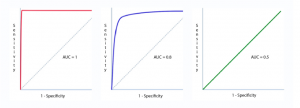
The Area under the ROC curve (AUC) is used to determine the model performance. The area under the ROC curve is a measure of the model’s ability to distinguish between the two classes. An AUC of 1 indicates a perfect classifier, while an AUC of 0.5 suggests no discriminative power, equivalent to random guessing. The following represents different ROC curves and related AOC values.

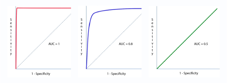
Figure: Sensitivity vs Specificity represented as ROC to determine AUC

The diagram below represents a scenario of high sensitivity (low false negatives) and low specificity (high false positives).

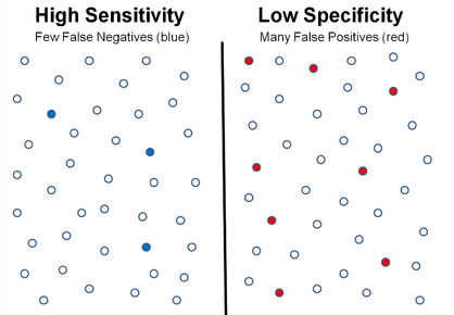
Figure: High Sensitivity vs Low Specificity

In general, a model with high sensitivity will have a high false-positive rate, while a model with high specificity will have a high false-negative rate. The trade-off between sensitivity and specificity can be tuned by changing the threshold for classification. A higher threshold will result in a model with high sensitivity and low specificity, while a lower threshold will result in a model with low sensitivity and high specificity.

Sensitivity & Specificity Python Code Example

In order to understand the concepts of sensitivity and specificity, let’s create a simple classification model using Python and a standard dataset. We’ll then evaluate its performance using sensitivity and specificity, among other metrics. The following is the step-by-step method for training and evaluating the model:

1. Dataset: Use a standard dataset suitable for classification, such as the Iris dataset or the Breast Cancer dataset from scikit-learn.
2. Model: Train a basic classification model, like a logistic regression or a decision tree.
3. Evaluation: Calculate sensitivity, specificity, and possibly other metrics like accuracy, precision, and the ROC curve.

For this demonstration, we will use the Breast Cancer dataset from scikit-learn, which is a binary classification problem well-suited for illustrating these concepts. Then, we’ll train a simple classifier and evaluate it.

from sklearn.datasets import load_breast_cancer
from sklearn.model_selection import train_test_split
from sklearn.linear_model import LogisticRegression
from sklearn.metrics import confusion_matrix, classification_report, roc_auc_score, roc_curve
import numpy as np

# Load the breast cancer dataset
data = load_breast_cancer()
X = data.data
y = data.target

# Split the dataset into training and test sets
X_train, X_test, y_train, y_test = train_test_split(X, y, test_size=0.3, random_state=42)

# Initialize and train the logistic regression model
model = LogisticRegression(max_iter=10000)
model.fit(X_train, y_train)

# Make predictions on the test set
y_pred = model.predict(X_test)
y_pred_prob = model.predict_proba(X_test)[:, 1]

# Calculate the confusion matrix
cm = confusion_matrix(y_test, y_pred)
tp, fn, fp, tn = cm.ravel()

# Calculate sensitivity and specificity
sensitivity = tp / (tp + fn)
specificity = tn / (tn + fp)

sensitivity, specificity, cm

The logistic regression model was trained on the Breast Cancer dataset and then evaluated on the test set. Here are the results:

• Sensitivity (True Positive Rate): Approximately 0.968, meaning the model correctly identifies about 96.8% of the actual positive cases.
• Specificity (True Negative Rate): Approximately 0.981, meaning the model correctly identifies about 98.1% of the actual negative cases.

The confusion matrix for this model is as follows:

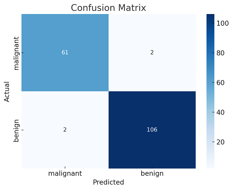
From the confusion matrix:

• 61 true positives (patients with cancer correctly identified)
• 106 true negatives (patients without cancer correctly identified)
• 2 false positives (patients without cancer incorrectly identified as having it)
• 2 false negatives (patients with cancer incorrectly identified as not having it)

These results indicate that the model performs quite well in both identifying the positive cases (sensitivity) and in avoiding false alarms (specificity).

Next, we will plot the ROC curve and calculate the AUC (Area Under Curve) to further assess the model’s performance.

import matplotlib.pyplot as plt

# Calculate the ROC Curve and AUC
fpr, tpr, thresholds = roc_curve(y_test, y_pred_prob)
roc_auc = roc_auc_score(y_test, y_pred_prob)

# Plotting the ROC Curve
plt.figure(figsize=(8, 6))
plt.plot(fpr, tpr, color='blue', lw=2, label=f'ROC curve (area = {roc_auc:.2f})')
plt.plot([0, 1], [0, 1], color='gray', lw=2, linestyle='--')
plt.xlim([0.0, 1.0])
plt.ylim([0.0, 1.05])
plt.xlabel('False Positive Rate')
plt.ylabel('True Positive Rate')
plt.title('Receiver Operating Characteristic (ROC) Curve')
plt.legend(loc="lower right")
plt.show()

Here is the plot for ROC curve:

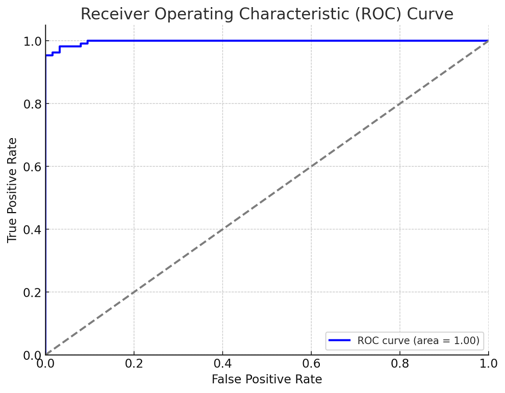
The Receiver Operating Characteristic (ROC) curve for the logistic regression model is displayed above, and it shows an excellent performance. The Area Under the Curve (AUC) is approximately 0.998, which is very close to the ideal value of 1. This high AUC value indicates that the model has a strong ability to distinguish between the two classes (presence and absence of breast cancer in this case).

In summary:

• The model has high sensitivity and specificity, indicating good performance in identifying positive cases and avoiding false positives.
• The ROC curve and the high AUC further confirm the model’s effectiveness in classification tasks.

This analysis demonstrates how sensitivity, specificity, and the ROC curve can be used to evaluate and understand the performance of a classification model, particularly in a medical diagnosis context

• Author
• Recent Posts

Follow me

Ajitesh Kumar

I have been recently working in the area of Data analytics including Data Science and Machine Learning / Deep Learning. I am also passionate about different technologies including programming languages such as Java/JEE, Javascript, Python, R, Julia, etc, and technologies such as Blockchain, mobile computing, cloud-native technologies, application security, cloud computing platforms, big data, etc. For latest updates and blogs, follow us on Twitter. I would love to connect with you on Linkedin.
Check out my latest book titled as First Principles Thinking: Building winning products using first principles thinking. Check out my other blog, Revive-n-Thrive.com

Follow me

Latest posts by Ajitesh Kumar (see all)

• Logistic Regression in Machine Learning: Python Example - April 26, 2024
• MSE vs RMSE vs MAE vs MAPE vs R-Squared: When to Use? - April 25, 2024
• Gradient Descent in Machine Learning: Python Examples - April 22, 2024