Have you ever faced a crucial decision where you needed to rely on data to guide your choice? Whether it’s determining the effectiveness of a new medical treatment or assessing the quality of a manufacturing process, hypothesis testing becomes essential. That’s where the Neyman-Pearson Lemma steps in, offering a powerful framework for making informed decisions based on statistical evidence.
The Neyman-Pearson Lemma holds immense importance when it comes to solving problems that demand decision making or conclusions to a higher accuracy. By understanding this concept, we learn to navigate the complexities of hypothesis testing, ensuring we make the best choices with greater confidence. In this blog post, we will explore the concepts of the Neyman-Pearson Lemma with the help of real-world examples and Python code example.
What is Neyman-Pearson Lemma?
From the hypothesis testing standpoint, the Neyman-Pearson Lemma stands as a fundamental principle that guides the construction of powerful statistical tests. By comprehending the key principles behind this lemma, we can enhance our ability to make informed decisions based on data.
The Neyman-Pearson Lemma states that the likelihood ratio test is the most powerful test for a given significance level (or size) in the context of simple binary hypothesis testing problems. It provides a theoretical basis for determining the critical region or decision rule that maximizes the probability of correctly detecting a true effect while maintaining a fixed level of Type I error (false positive rate).
At the heart of the Neyman-Pearson Lemma lies the concept of statistical power. Statistical power represents the ability of a hypothesis test to detect a true effect or difference when it exists in the population. The lemma emphasizes the importance of optimizing this power while controlling the risk of both Type I and Type II errors.
Type I error, also known as a false positive, occurs when we reject the null hypothesis (assuming an effect or difference exists) when it is actually true. Type II error, on the other hand, refers to a false negative, where we fail to reject the null hypothesis (assuming no effect or difference) when an effect or difference truly exists. The Neyman-Pearson Lemma allows us to strike a balance between these errors by maximizing power while setting a predetermined significance level (the probability of Type I error).
By employing the Neyman-Pearson Lemma, we can design tests that optimize statistical power while controlling the rate of false positives. This ensures that we have a greater chance of correctly identifying true effects or differences in our data. Understanding the foundations of the Neyman-Pearson Lemma empowers us to make informed decisions backed by robust statistical analyses. In the upcoming sections, we will explore practical examples that illustrate the application of this lemma in various fields, further solidifying our understanding of its significance.
Note that in Neyman-Pearson Lemma, “lemma” refers to a mathematical term. In mathematics, a lemma is a proven statement or proposition that serves as a stepping stone or auxiliary result in the proof of a larger theorem. The Neyman-Pearson Lemma itself is a theorem in hypothesis testing theory, and it is named after the statisticians Jerzy Neyman and Egon Pearson, who developed it independently in the 1920s and 1930s. The lemma serves as a crucial intermediate result in the derivation and understanding of hypothesis testing procedures.
Here is the summary of what we learned so far about Neyman-Pearson Lemma:
- The Neyman-Pearson Lemma guides the construction of powerful statistical tests in hypothesis testing.
- It states that the likelihood ratio test is the most powerful test for a given significance level in binary hypothesis testing.
- Statistical power is emphasized, representing the ability to detect true effects while controlling errors.
- The lemma balances Type I and Type II errors by optimizing power under a predetermined significance level.
- Employing the Neyman-Pearson Lemma enables tests with higher chances of correctly identifying true effects.
How does Neyman-Pearson Lemma work?
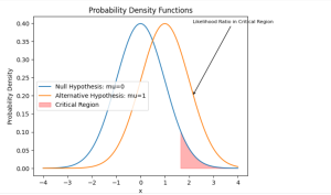
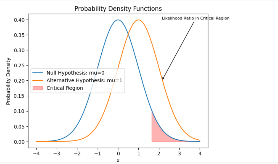
In order to understand how Neyman-Pearson works, lets consider a binary hypothesis testing problem with two hypotheses: a null hypothesis (H0) and an alternative hypothesis (H1). Let’s denote the probability density functions (pdfs) of the observed data under the null and alternative hypotheses as f0(x) and f1(x), respectively. The Neyman-Pearson lemma states that the likelihood ratio test is the most powerful test for a fixed significance level α.
The likelihood ratio test compares the likelihoods of the observed data under the null and alternative hypotheses and accepts the alternative hypothesis if the likelihood ratio exceeds a certain threshold. Mathematically, the likelihood ratio test is given by:
Reject H0 if L(x) = f1(x) / f0(x) > k
where k is a threshold determined based on the desired significance level α. The threshold k is chosen such that the probability of Type I error (false positive) is equal to α.
The Neyman-Pearson lemma states that the likelihood ratio test has the highest statistical power among all tests with the same significance level α. In other words, it maximizes the probability of detecting a true effect or rejecting the null hypothesis when the alternative hypothesis is true.
It’s important to note that the Neyman-Pearson lemma assumes that the null and alternative hypotheses are simple, meaning they are completely specified (e.g., specific parameter values) and mutually exclusive. In practice, the lemma is often used as a basis for constructing tests in more general settings, such as composite hypotheses or hypothesis tests involving multiple parameters.
The Neyman-Pearson lemma provides a theoretical foundation for hypothesis testing, and its concepts are widely used in statistical inference and decision-making.
Neyman-Pearson Lemma Real-world Example
One real-world example where the Neyman-Pearson lemma test can be used is in medical testing, specifically for diagnosing a disease. Let’s consider a hypothetical scenario:
Null hypothesis (H0): The patient does not have the disease.
Alternative hypothesis (H1): The patient has the disease.
In this example, we want to design a test that can accurately determine whether a patient has a specific disease or not. We need to balance the risks of two types of errors:
Type I error (false positive): Rejecting the null hypothesis (saying the patient has the disease) when the patient is actually healthy.
Type II error (false negative): Failing to reject the null hypothesis (saying the patient is healthy) when the patient actually has the disease.
To apply the Neyman-Pearson lemma, we would need to determine the likelihood ratio test based on the data and find a threshold that controls the significance level of the test (the probability of a Type I error). For example, suppose we have collected data on a specific biomarker that is known to be associated with the disease. We can model the biomarker levels for healthy patients (H0) as a normal distribution with a certain mean and variance, and the biomarker levels for patients with the disease (H1) as another normal distribution with a different mean and variance.
The null hypothesis (H0) would be formulated as: The biomarker levels follow a normal distribution with parameters μ0 (mean under H0) and σ0 (variance under H0).
The alternative hypothesis (H1) would be formulated as: The biomarker levels follow a normal distribution with parameters μ1 (mean under H1) and σ1 (variance under H1), where μ1 > μ0.
To perform the hypothesis test, we would calculate the likelihood ratio, which is the ratio of the likelihood of the observed data under the alternative hypothesis to the likelihood under the null hypothesis. If the likelihood ratio exceeds a certain threshold (determined based on the desired significance level), we would reject the null hypothesis in favor of the alternative hypothesis.
The Neyman-Pearson lemma guarantees that this likelihood ratio test will have the highest statistical power (i.e., the highest probability of correctly detecting the disease when it is present) among all tests with the same significance level.
In practice, medical researchers and practitioners would collect data, estimate the parameters of the null and alternative hypotheses (e.g., using maximum likelihood estimation), and then perform the likelihood ratio test to make informed decisions about the presence or absence of the disease in individual patients.
Neyman-Pearson Lemma Python Example
While the Neyman-Pearson lemma is a theoretical concept, I can provide you with a Python code example that demonstrates the implementation of the likelihood ratio test based on the Neyman-Pearson lemma for a simple hypothesis testing problem. Let’s consider a scenario of testing the mean of a normal distribution.
import numpy as np
from scipy.stats import norm

# Generate sample data
np.random.seed(0)
n = 100  # Number of samples
mu0 = 0  # Null hypothesis mean
mu1 = 1  # Alternative hypothesis mean
sigma = 1  # Common standard deviation
data = np.random.randn(n) + mu1  # Samples from the alternative distribution

# Compute likelihood ratio test
likelihood_ratio = np.prod(norm.pdf(data, mu1, sigma)) / np.prod(norm.pdf(data, mu0, sigma))
print("Likelihood ratio = ", likelihood_ratio)


# Set significance level and threshold
alpha = 0.05  # Significance level
threshold = norm.ppf(1 - alpha)  # Threshold based on significance level
print("Threshold, k = ", threshold)

# Perform hypothesis test
if likelihood_ratio > threshold:
    print("Reject null hypothesis")
else:
    print("Fail to reject null hypothesis")
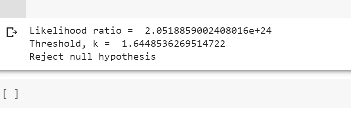
The following gets printed:
In this example, we first generate a sample dataset by drawing samples from a normal distribution with a mean of mu1 (alternative hypothesis) and a standard deviation of sigma. We assume that the null hypothesis is a normal distribution with a mean of mu0. The likelihood_ratio is computed by calculating the likelihood of the data under the alternative hypothesis divided by the likelihood under the null hypothesis.
We then set the desired significance level alpha (e.g., 0.05) and calculate the threshold (critical region) for rejecting the null hypothesis based on the inverse cumulative distribution function (CDF) of the standard normal distribution(norm.ppf). If the likelihood_ratio exceeds the threshold (critical region), we reject the null hypothesis; otherwise, we fail to reject the null hypothesis. In the above example, we rejected the null hypothesis as likelihood ratio (2.0519) exceeded the threshold value (1.6448). The same is demonstrated below.
In the above code example, norm.pdf(data, mu1, sigma) is a function call that computes the probability density function (PDF) of the normal distribution at the given randomly generated data points (np.random.randn(n) + mu1), assuming a specific mean mu1 (alternative hypothesis) and standard deviation sigma. Similarly, norm.pdf(data, mu0, sigma) computes the PDF of the normal distribution at the given data points, assuming a specific mean mu0 (null hypothesis) and standard deviation sigma.
Conclusion
The Neyman-Pearson Lemma provides a principled approach to designing powerful statistical tests. By understanding the foundations of this lemma, we gained valuable insights into optimizing statistical power while controlling error rates. The ability to strike a balance between Type I and Type II errors empowers us to make informed decisions based on data, ensuring that we correctly identify true effects or differences. From medical research to quality control and beyond, the Neyman-Pearson Lemma finds widespread application in various fields where robust hypothesis testing is paramount. By harnessing its principles, we equip ourselves with a valuable tool to navigate the complexities of statistical inference and make sound judgments backed by rigorous analyses.

Check out my latest book titled as First Principles Thinking: Building winning products using first principles thinking.
- Mathematics Topics for Machine Learning Beginners - July 6, 2025
- Questions to Ask When Thinking Like a Product Leader - July 3, 2025
- Three Approaches to Creating AI Agents: Code Examples - June 27, 2025
I found it very helpful. However the differences are not too understandable for me