The confusion matrix is an essential tool in the field of machine learning and statistics for evaluating the performance of a classification model. It’s particularly useful when dealing with binary or multi-class classification problems. In this post, you will learn about the confusion matrix with examples and how it could be used as performance metrics for classification models in machine learning.
What is Confusion Matrix?
A confusion matrix is a table used to describe the performance of a classification model on a set of test data for which the true values are known. It’s most useful when you need to know more about the accuracy of the model than just the overall accuracy.
In the simplest case, for a binary classification problem, the confusion matrix consists of four different combinations of predicted and actual values:
- True Positives (TP): The cases in which the model correctly predicted the positive class.
- True Negatives (TN): The cases in which the model correctly predicted the negative class.
- False Positives (FP): The cases in which the model incorrectly predicted the positive class (also known as a Type I error).
- False Negatives (FN): The cases in which the model incorrectly predicted the negative class (also known as a Type II error).
Why is Confusion Matrix useful?
The following are some of the reasons why confusion matrix is very useful and dat scientists must get a good hold on this concept:
-
Performance Measures: Beyond simple accuracy (which can be misleading, especially in unbalanced datasets), the confusion matrix allows calculation of various performance metrics like precision, recall, F1 score, specificity, etc. Each of these metrics gives different insights into the strengths and weaknesses of the model.
-
Insight into Errors: It provides insights into the types of errors the model is making. For instance, in medical diagnosis, a false negative might be more dangerous than a false positive.
-
Handling Imbalanced Datasets: In cases where class distribution is not balanced, the confusion matrix helps in assessing the model performance for each class separately.
-
Model Tuning: Understanding the types of errors and their quantities can guide you in tuning your model. For example, if there are too many false positives, you might want to increase the threshold for predicting the positive class.
Real-world Example of Confusion Matrix
Let’s take a real-world example of a loan default classification model. In this scenario, the model aims to predict whether a borrower will default on a loan (i.e., fail to repay it) based on various factors like credit score, income, loan amount, etc.
The historical data was gathered for the borrowers, including whether they defaulted and other relevant features. The data was used to train a classification model (say a logistic regression model) to predict default. The model was evaluated on a separate test dataset consisting of 1000 borrowers to see how well it predicts loan defaults.
Let’s say the following was the result:
- True Positives (TP): 150
- True Negatives (TN): 700
- False Positives (FP): 50
- False Negatives (FN): 100
The confusion matrix for this example would look like this:
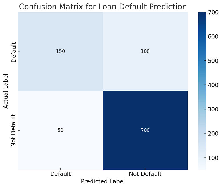
The following is how the above confusion matrix can be interpreted:
- TP (150): The model correctly identified 150 borrowers who defaulted.
- TN (700): The model correctly identified 700 borrowers who did not default.
- FP (50): The model incorrectly identified 50 borrowers as likely to default, but they did not.
- FN (100): The model missed 100 borrowers who did default, predicting that they would not.
Python Code Example for Confusion Matrix
In this section, you will see the Sklearn Python code example of confusion matrix. The model below is trained using the support vector classifier (SVC) algorithm. Sklearn.svm package is used for importing SVC. The following are some of the aspects illustrated in the code example given below:
- Sklearn IRIS dataset is used for training the model
- train_test_split method is used for creating the training and test data split.
- StandardScaler instance is used for data standardization
- SVC algorithm is used for fitting the model
- Sklearn.metrics confusion_matrix is used for calculating the confusion matrix.
Here is how the code will look like
from sklearn.datasets import load_iris
from sklearn.model_selection import train_test_split
from sklearn.svm import SVC
from sklearn.metrics import confusion_matrix
import seaborn as sns

# Load Iris dataset
iris = load_iris()
X = iris.data
y = iris.target

# Split the dataset into training and testing sets
X_train, X_test, y_train, y_test = train_test_split(X, y, test_size=0.3, random_state=42)

# Train an SVC model
svc = SVC(gamma='auto')
svc.fit(X_train, y_train)

# Make predictions
y_pred = svc.predict(X_test)

# Construct the confusion matrix
conf_matrix_iris = confusion_matrix(y_test, y_pred)

# Plotting the confusion matrix
plt.figure(figsize=(8, 6))
sns.heatmap(conf_matrix_iris, annot=True, fmt="d", cmap="Blues",
            xticklabels=iris.target_names, yticklabels=iris.target_names)

# Adding labels and title
plt.ylabel('Actual Label')
plt.xlabel('Predicted Label')
plt.title('Confusion Matrix for Iris Dataset (SVC Model)')

plt.show()
Here is how the confusion matrix would look like:

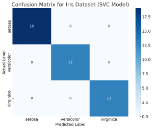
The above shown image is the confusion matrix for the Iris dataset, using a Support Vector Classifier (SVC). The matrix is constructed from the predictions made on the test set.
In this matrix:
- The rows represent the actual classes of the Iris dataset (setosa, versicolor, virginica).
- The columns represent the predicted classes by the SVC model.
Each cell shows the number of instances of the actual class (row) that were predicted as a certain class (column). For example, a cell at the intersection of “versicolor” actual and “virginica” predicted would show the number of times the model incorrectly predicted a versicolor iris as virginica.
This confusion matrix provides a clear view of how well the model is performing for each class, indicating any biases or tendencies in its predictions

Check out my latest book titled as First Principles Thinking: Building winning products using first principles thinking.
- Mathematics Topics for Machine Learning Beginners - July 6, 2025
- Questions to Ask When Thinking Like a Product Leader - July 3, 2025
- Three Approaches to Creating AI Agents: Code Examples - June 27, 2025
I found it very helpful. However the differences are not too understandable for me