One of the common challenges faced with the deployment of large language models (LLMs) while achieving low-latency completions (inferences) is the size of the LLMs. The size of LLM throws challenges in terms of compute, storage, and memory requirements. And, the solution to this is to optimize the LLM deployment by taking advantage of model compression techniques that aim to reduce the size of the model. In this blog, we will look into three different optimization techniques namely pruning, quantization, and distillation along with their examples. These techniques help model load quickly while enabling reduced latency during LLM inference. They reduce the resource requirements for the compute, storage, and memory. You might want to check out the book Generative AI on AWS to learn how to apply this technique on the AWS cloud.
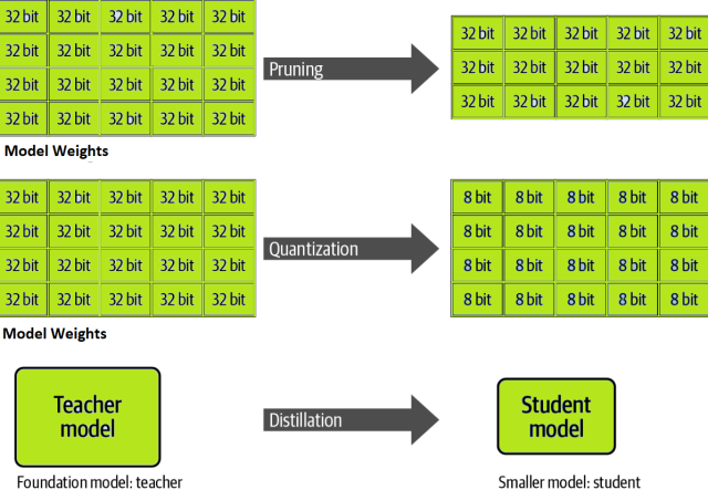
The following diagram represents different optimization techniques for LLM inference such as Pruning, Quantization, and Distillation.
Let’s learn about the LLM inference optimization techniques in detail in the following sections with the help of examples.
Pruning – Eliminate Parameters
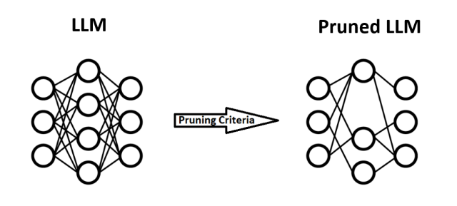
Pruning is a technique that aims to reduce the model size of LLM by removing the weights that contribute minimally to the output. This is based on the observation that not all parameters used in LLM are equally important for making predictions. By identifying and eliminating these low-impact parameters, pruning reduces the model’s size and the number of computations required during inference, leading to faster and more efficient performance. The following diagram represents the pruned LLM after some weights have been removed.
There are various strategies for pruning, including magnitude-based pruning (unstructured pruning), where weights with the smallest absolute values are pruned, and structured pruning, which removes entire channels or filters based on their importance. Pruning can be applied iteratively, with cycles of pruning followed by fine-tuning to recover any lost performance, resulting in a compact model that retains much of the original model’s accuracy.
The above-mentioned approaches (structured and unstructured pruning) require retraining; however, there are post-training pruning methods as well. These methods are typically referred to as one-shot pruning methods. These methods can do pruning without retraining. One such method of post-training pruning is called SparseGPT. This technique has been found to achieve pruning of magnitude to at least 50% sparsity in one-shot, without any retraining, at minimal loss of accuracy. The following code sample from the SparseGPT pruning library demonstrates how pruning is achieved for the LLaMA and Llama 2 models.
target_sparsity_ratio = 0.5

# Prune each layer using the given sparsity ratio
for layer_name in layers:
  gpts[layer_name].fasterprune(
    target_sparsity_ratio,
  )

gpts[layer_name].free() # free the zero'd out memory
Quantization – Model Weights Precision Conversion
In the Quantization technique, the model’s weights are converted from high precision (e.g., 32-bit) to lower precision (e.g., 16-bit). This not only reduces the model’s memory footprint but also the compute requirements by working with a smaller number of representations. With large LLMs, it’s common to reduce the precision further to 8 bits to increase inference performance. The popular method of quantization is reducing the precision of a model’s weights and activations after it has already been trained, as opposed to applying quantization during the training process itself. This method is also called post-training quantization (PTQ). The PTQ method is a popular option for optimizing models for inference because it doesn’t require retraining the model from scratch with quantization-aware techniques.
There are a variety of post-training quantization methods, including GPT post-training quantization (GPTQ). Check out this paper for the details – GPTQ: Accurate Post-Training Quantization for Generative Pre-trained Transformers.
Distillation – Statistical Method for Training Smaller Model
Distillation is an LLM model optimization technique for inference that helps reduce the model size thereby reducing the number of computations. It uses statistical methods to train a smaller student model on a larger teacher model. The result is a student model that retains a high percentage of the teacher’s model accuracy but uses a much smaller number of parameters. The student model is then deployed for inference.
The teacher model is often a generative pre-trained / foundation or a fine-tuned LLM. During the distillation training process, the student model learns to statistically replicate the behavior of the teacher model. Both the teacher and student models generate completions from a prompt-based training dataset. A loss function is calculated by comparing the two completions and calculating the KL divergence between the teacher and student output distributions. The loss is then minimized during the distillation process using backpropagation to improve the student model’s ability to match the teacher model’s predicted next-token probability distribution.
A popular distilled student model is DistilBERT from Hugging Face. DistilBERT was trained from the larger BERT teacher model and is an order of magnitude smaller than BERT, yet it retains approximately 97% of the accuracy of the original BERT model.
Conclusion
Each of these optimization techniques—pruning, quantization, and distillation—offers a pathway to optimizing LLMs for inference, making them more accessible for deployment in resource-constrained environments. The choice of technique(s) depends on the specific requirements and constraints of the deployment scenario, such as the acceptable trade-off between accuracy and computational efficiency, the hardware available for inference, and the specific tasks the LLM is being used for. Often, a combination of these techniques is employed to achieve an optimal balance.
- The Watermelon Effect: When Green Metrics Lie - January 25, 2026
- Coefficient of Variation in Regression Modelling: Example - November 9, 2025
- Chunking Strategies for RAG with Examples - November 2, 2025


I found it very helpful. However the differences are not too understandable for me