If you’re working with data analytics projects including building machine learning (ML) models, you’ve probably heard of the K-nearest neighbors (KNN) algorithm. But what is it, exactly? And more importantly, how can you use it in your own AI / ML projects? In this post, we’ll take a closer look at the KNN algorithm and walk through a simple Python example. You will learn about the K-nearest neighbors algorithm with Python Sklearn examples. K-nearest neighbors algorithm is used for solving both classification and regression machine learning problems. Stay tuned!
Introduction to K-Nearest Neighbors (K-NN) Algorithm
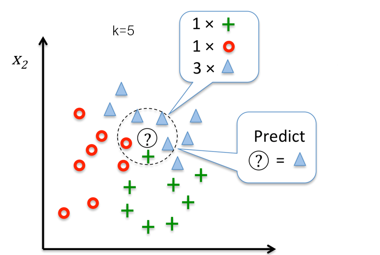
K-nearest neighbors is a supervised machine learning algorithm for classification and regression. In both cases, the input consists of the k closest training examples in the feature space. The output depends on whether k-nearest neighbors are used for classification or regression. The main idea behind K-NN is to find the K nearest data points, or neighbors, to a given data point and then predict the label or value of the given data point based on the labels or values of its K nearest neighbors. K can be any positive integer, but in practice, K is often small, such as 3 or 5. The “K” in K-nearest neighbors refers to the number of items that the algorithm uses to make its prediction whether its a classification problem or a regression problem. The following diagram represents how K nearest neighbors are used for making predictions.

The following are key aspects of K-nearest neighbor’s algorithms.
- In the k-nearest neighbor’s classification, the output is a class membership. An object is classified by a majority vote of its neighbors, with the object being assigned to the class most common among its k nearest neighbors (k is a positive integer, typically small). If k = 1, then the object is simply assigned to the class of that single nearest neighbor.
- In the K-nearest neighbors regression, the output is the property value for the object. This value is the average of the values of its k nearest neighbors.
K-nearest neighbor is a non-parametric method, which means that it does not make any assumptions about the underlying data. This is advantageous over parametric methods, which do make such assumptions. The models don’t learn parameters from the training data set to come up with a discriminative function in order to classify the test or unseen data set. Rather model memorizes the training data set. This is why the K-NN classifier is also called a lazy learner. Here is what is done as part of the algorithm to classify the data:
- First and foremost, the value of K and distance metric is selected. The value of K represents the number of nearest data points that would be selected for making the prediction. Distance metric would be used to measure the similarity of the data points. The distance metric typically used is Euclidean distance. Read about some of the most popular distance metric measures in this post – Different types of distance measures in machine learning. In SKlearn KNeighborsClassifier, the distance metric is specified using the parameter metric. The default value of the metric is Minkowski. Another parameter is p. With the value of metric as Minkowski, the value of p = 1 means Manhattan distance and the value of p = 2 means Euclidean distance.
- Once K and distance metric are selected, K-NN algorithm goes through the following steps:
- Calculate distance: The K-NN algorithm calculates the distance between a new data point and all training data points. This is done using the selected distance metric.
- Find nearest neighbors: Once distances are calculated, K-nearest neighbors are determined based on a set value of K.
- Predict target class label: After finding out K nearest neighbors, we can then predict the target class label for a new data point by taking majority vote from its K neighbors (in case of classification) or by taking average from its K neighbors (in case of regression).
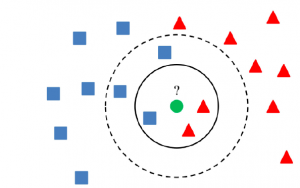
In the diagram below, if K = 3, the class of the data point (green) is assigned as the orange triangle (2 votes to 1 in favor of the orange triangle). If K = 5, the class of the data point gets assigned as blue square (3 votes to 2 votes in favor of blue square).

The advantages of using K-NN algorithm to train the models are some of the following:
- K-NN is a very simple algorithm to understand and implement.
- K-NN can be used for both classification and regression problems.
- K-NN works well with small dataset as well as large dataset.
- K-NN does not make any assumptions on the data distribution, which is an advantage over other parametric methods such as logistic regression and linear discriminant analysis.
- K-NN is also not sensitive to outliers in the data.
The disadvantages of K-NN algorithm are some of the following:
- K-NN requires a large amount of memory to store all training data points since we need to calculate the distance between a new data point and all training data points. This can be problematic when working with large datasets.
- Another disadvantage of K-NN is that it can be computationally expensive to calculate the distance between a new data point and all training data points.
- K-NN might not work well with high dimensional data since the distance metric can become distorted in higher dimensions.
What is the most appropriate value of K in K-NN?
It is of utmost importance to choose the appropriate value of K in order to avoid issues related to overfitting or underfitting. Note that for a larger value of K, the model may underfit and for a smaller value of K, the model may overfit. Thus, it is of utmost importance to choose the most appropriate value of K. You may want to check out this post to have a good understanding of underfitting and overfitting concepts. One can draw a validation curve to assess the same. Here are some strategies which can be used for selecting the most appropriate value of K.
- Using coprime class and K combinations: Coprime numbers are the numbers that don’t share common divisors other than 1. For example, 8 and 15 or 3 and 4. Thus, if there are 3 classes, then the value or K can be 2 or 4 or 5 or 7 or 8, etc.
- Choosing the value of K which is greater or equal to the number of classes plus 1
- K = No of Classes + 1
- Choosing the value of K which is low enough to avoid noise; When using a larger value of K can result in high model bias. At the same time, keep in mind that choosing a very less value of K can result in high variance or overfitting.
K-NN Python Sklearn Example
Here is the Python Sklearn code for training the model using K-nearest neighbors. Two different versions of the code are presented. One is the very simplistic way. Another is using pipeline and grid search.
Simplistic Python Code for Fitting K-NN Model
Here is the simplistic code for fitting the K-NN model using the Sklearn IRIS dataset. Pay attention to some of the following in the code given below:
- Sklearn.model_selection train_test_split is used for creating training and test split data
- Sklearn.preprocessing StandardScaler (fit & transform method) is used for feature scaling.
- Sklearn.neighbors KNeighborsClassifier is used as implementation for the K-nearest neighbors algorithm for fitting the model. The following are some important parameters for K-NN algorithm:
- n_neighbors: Number of neighbors to use
- weights: Weight is used to associate the weight assigned to points in the neighborhood. If the value of weights is “uniform”, it means that all points in each neighborhood are weighted equally. If the value of weights is “distance”, it means that closer neighbors of a query point will have a greater influence than neighbors which are further away.
from sklearn.neighbors import KNeighborsClassifier
from sklearn.preprocessing import StandardScaler
from sklearn.pipeline import make_pipeline
from sklearn import datasets
from sklearn.model_selection import train_test_split
from sklearn.metrics import accuracy_score
from sklearn.model_selection import GridSearchCV
#
# Load the Sklearn IRIS dataset
#
iris = datasets.load_iris()
X = iris.data
y = iris.target
#
# Create train and test split
#
X_train, X_test, y_train, y_test = train_test_split(X, y, test_size=0.3, random_state=42, stratify=y)
#
# Feature Scaling using StandardScaler
#
sc = StandardScaler()
sc.fit(X_train)
X_train_std = sc.transform(X_train)
X_test_std = sc.transform(X_test)
#
# Fit the model
#
knn = KNeighborsClassifier(n_neighbors=5, p=2, weights='uniform', algorithm='auto')
knn.fit(X_train_std, y_train)
#
# Evaluate the training and test score
#
print('Training accuracy score: %.3f' % knn.score(X_train_std, y_train))
print('Test accuracy score: %.3f' % knn.score(X_test_std, y_test))
The model score for the training data set comes out to be 0.981 and the test data set is 0.911. Let’s take a look at the usage of pipeline and gridsearchcv for training / fitting the K-NN model
Pipeline and GridSearchCV for fitting the K-NN model
Here is the code for fitting the model using Sklearn K-nearest neighbors implementation. Pay attention to some of the following:
- Sklearn.pipeline make_pipeline is used for creating a pipeline having steps including StandardScaler and KNeighborsClassifier
- GridSearchCV is used for tuning model parameters and selecting the best estimator with the most optimal score
#
# Load the Sklearn IRIS dataset
#
iris = datasets.load_iris()
X = iris.data
y = iris.target
#
# Create train and test split
#
X_train, X_test, y_train, y_test = train_test_split(X, y, test_size=0.3, random_state=42, stratify=y)
#
# Create a pipeline
#
pipeline = make_pipeline(StandardScaler(), KNeighborsClassifier())
#
# Create the parameter grid
#
param_grid = [{
    'kneighborsclassifier__n_neighbors': [2, 3, 4, 5, 6, 7, 8, 9, 10],
    'kneighborsclassifier__p': [1, 2],
    'kneighborsclassifier__weights': ['uniform', 'distance'],
    'kneighborsclassifier__algorithm': ['auto', 'ball_tree', 'kd_tree', 'brute'],
}]
#
# Create a grid search instance
#
gs = GridSearchCV(pipeline, param_grid = param_grid,
                  scoring='accuracy',
                  refit=True,
                  cv=10,
                  verbose=1,
                  n_jobs=2)
#
# Fit the most optimal model
#
gs.fit(X_train, y_train)
#
# Print the best model parameters and scores
#
print('Best Score: %.3f' % gs.best_score_, '\nBest Parameters: ', gs.best_params_)
#
# Print the model score for test data
#
print('Score: %.3f' % gs.score(X_test, y_test))
The score of the test data set comes out to be 0.911 and the training data comes out to be 0.972. Here is what the output looks like after executing the above code.

Some Good Youtube Tutorials on K-Nearest Neighbors
Statquest: K-nearest neighbors, clearly explained
How K-NN algorithm works?
Conclusions
Here is the summary of what you learned in relation to the K-nearest Neighbors Classifier:
- K-NN algorithm belongs to a non-parametric class of machine learning algorithms.
- In the K-NN algorithm, K represents the number of data points that need to be chosen for making the predictions.
- Out of K data points selected for prediction, the voting takes place in terms of how many of them belongs to which class. Based on that, the class of the data gets decided.
- It is recommended to select the odd value of K for binary classification
- It is recommended that the value of K should not be a multiple of a number of classes.
- One can opt for either Euclidean or Manhattan distance for measuring the similarity between the data points. For Sklearn KNeighborsClassifier, with metric as Minkowski, the value of p = 1 means Manhattan distance and the value of p = 2 means Euclidean distance. The default is Euclidean distance with metric = ‘minkowski’ and p = 2.
- For real-world examples, often Euclidean distance is used. However, it is recommended to standardize the data set beforehand.
- Mathematics Topics for Machine Learning Beginners - July 6, 2025
- Questions to Ask When Thinking Like a Product Leader - July 3, 2025
- Three Approaches to Creating AI Agents: Code Examples - June 27, 2025
I found it very helpful. However the differences are not too understandable for me