
Learning the concepts of Minimum Description Length (MDL) is valuable for several reasons, especially for those involved in statistics, machine learning, data science, and related fields. One of the fundamental problems in statistics and data analysis is choosing the best model from a set of potential models. The challenge is to find a model that captures the essential features of the data without overfitting. This is where methods such as MDL, AIC, BIC, etc. comes to rescue. MDL offers a principled way to balance model complexity against the goodness of fit. This is crucial in many areas, such as machine learning and statistical modeling, where overfitting is a common problem. Understanding MDL provides several benefits related to model selection, generalization to new data, strengthening theoretical foundation linked to the core principles of information theory, etc. In this blog, we will learn about concepts of MDL, how it could be applied to solve real-world problems with the help of examples.
Understanding Minimum Description Length (MDL) Concepts
The Minimum Description Length (MDL) principle is a method in information theory and statistics for inductive inference, particularly for model selection. It’s based on the idea that the best explanation, or model, for a set of data is the one that minimizes the total length of the description of the model and the data given the model. This principle can be seen as a formalization of Occam’s Razor in the context of model selection.
The following are the core concepts related to MDL:
- Description Length: This is the core of the MDL principle. The description length involves two parts:
- The length of the description of the model (complexity of the model).
- The length of the data when encoded with the model (how well the model fits the data).
- Compression and Regularity: The MDL principle is grounded in the concept that any regularity in the data can be used to compress it. If a model can capture these regularities, it can describe the data more concisely. Let’s understand this with an example. Imagine you have two text files composed of sequences of characters:
- File A: Contains a long sequence of the same character repeated, like “AAAAAA….” (a very regular pattern).
- File B: Contains a random mix of characters with no discernible pattern, like “XpQr5Z…”.
- Applying MDL principle:
- Observing Regularities:
- File A: Exhibits a clear, simple pattern (repetition of ‘A’)
- File B: Shows no obvious pattern or regularity
- Modeling for Compression:
- Simple Model: A basic compression algorithm that looks for and compresses repeated characters.
- Complex Model: A more sophisticated algorithm that tries to find and encode more complex patterns.
- MDL Analysis:
- For File A: The simple model can compress it effectively by just noting the repeated ‘A’ character (e.g., “A repeated 1000 times”). The complex model wouldn’t offer much advantage and would add unnecessary complexity.
- For File B: The simple model can’t compress it effectively because there are no simple repeats. The complex model might also struggle due to the lack of patterns.
- MDL Decision:
- For File A, the simple model has a lower MDL since it provides sufficient compression with lower complexity.
- For File B, neither model may perform well, but the simple model might still be preferred due to its lower complexity, unless the complex model can find some less obvious patterns to compress.
- Observing Regularities:
- Trade-off Between Model Complexity and Fit: Simple models may not fit the data well, requiring a longer description of the residuals (the part of the data not explained by the model). Complex models may fit the data better but require a longer description themselves. The MDL seeks a balance between these two.
Let’s understand the concept of description length.
Description Length
To mathematically explain the concept of Description Length in the Minimum Description Length (MDL) principle, we’ll break it down into its two main components and discuss how each can be quantified.
Length of the Description of the Model (Model Complexity)
This component represents the cost of specifying the model. In mathematical terms, it’s often related to the number of parameters in the model or the complexity of the model structure. There are several ways to quantify this:
- Parametric Models: For models defined by parameters (like a linear regression model), the complexity can be related to the number of parameters. For example, in a linear regression model y=ax+b, there are two parameters (a and b), so the complexity might be considered as 2 units (assuming a fixed cost per parameter).
- Non-parametric Models: For models not defined by a fixed set of parameters (like decision trees), the complexity might be quantified by the size of the model structure (e.g., the number of nodes in a tree).
Mathematically, the model complexity (Cm) might be represented as:
Cm=f(model parameters or structure)
where f is a function that quantifies complexity.
Length of the Data When Encoded with the Model (Data Fit)
This component is about how well the model compresses or explains the data. It’s often quantified using the likelihood of the data given the model, which can be transformed into a length measure using information-theoretic concepts.
- Likelihood: The likelihood of the data given the model (often denoted L) measures how well the model explains the data. In information theory, the negative logarithm of the likelihood is used to represent information content.
- Information Content: For a given dataset D and a model M, the cost of encoding the data given the model can be expressed as the negative log-likelihood: Cd =−log(L(D∣M)) This represents the number of bits needed to encode the data given the model (assuming optimal encoding based on the model).
Total Description Length
The total description length (DL) in the MDL framework is the sum of these two components:
DL = Cm+Cd
This total length represents the overall cost of both describing the model and encoding the data using that model. The goal in MDL is to minimize this total description length, striking a balance between a simple model (lower Cm) and a good fit to the data (lower Cd).
Model Selection with MDL – Python Example
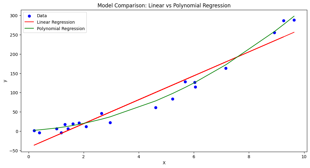
In this section, we will learn about how to use the Minimum Description Length (MDL) principle for model selection with a Python example. We’ll use a simple dataset and compare two models: a linear regression and a polynomial regression. Our goal will be to select the model that best balances complexity and data fit according to the MDL principle.
We’ll generate a synthetic dataset that follows a quadratic pattern with some noise. Then, we’ll fit two models to this data:
- Linear Regression Model (Model A): A simple model with lower complexity but potentially poorer fit.
- Polynomial Regression Model (Model B): A more complex model with a potentially better fit.
The following steps will be taken for model selection using MDL:
- Fit Models: Fit both a linear regression model and a polynomial regression model to the data.
- Calculate MDL for Each Model:
- Model Complexity: We’ll use the number of parameters as a proxy for model complexity.
- Data Fit: We’ll use the negative log-likelihood (or a related measure like mean squared error) to assess the fit.
- Select the Best Model: The model with the lower MDL is preferred.
import numpy as np
import matplotlib.pyplot as plt
from sklearn.linear_model import LinearRegression
from sklearn.preprocessing import PolynomialFeatures
from sklearn.metrics import mean_squared_error
from sklearn.model_selection import train_test_split

# Step 1: Generate Synthetic Data
np.random.seed(0)
X = np.random.rand(100, 1) * 10  # Random data points
y = 3 * X**2 + 2 * X + 1 + np.random.randn(100, 1) * 10  # Quadratic equation with noise

# Splitting the data into training and testing sets
X_train, X_test, y_train, y_test = train_test_split(X, y, test_size=0.2, random_state=0)

# Step 2: Fit Models
# Linear Regression Model
lin_reg = LinearRegression()
lin_reg.fit(X_train, y_train)
y_pred_lin = lin_reg.predict(X_test)

# Polynomial Regression Model
poly_features = PolynomialFeatures(degree=2, include_bias=False)
X_poly_train = poly_features.fit_transform(X_train)
X_poly_test = poly_features.transform(X_test)
poly_reg = LinearRegression()
poly_reg.fit(X_poly_train, y_train)
y_pred_poly = poly_reg.predict(X_poly_test)

# Step 3: Calculate MDL for Each Model
# Using Mean Squared Error as a proxy for negative log-likelihood

# Model A: Linear Regression
mdl_lin = 2 + mean_squared_error(y_test, y_pred_lin)  # 2 parameters (slope, intercept)

# Model B: Polynomial Regression
mdl_poly = 3 + mean_squared_error(y_test, y_pred_poly)  # 3 parameters (quadratic, linear, intercept)

(mdl_lin, mdl_poly)
The following is output by executing the code.
(578.3917388008515, 105.85467801527344)
The above output represents the Minimum Description Length (MDL) values for the two models we considered: the linear regression model (Model A) and the polynomial regression model (Model B). The values are:
- Linear Regression Model (Model A): MDL = 578.39
- Polynomial Regression Model (Model B): MDL = 105.85
Analysis of the Output
- Polynomial Regression Model (Lower MDL):
- With an MDL of 105.85, the polynomial model has a significantly lower description length compared to the linear model. This suggests that, despite being more complex (having more parameters), it does a much better job of fitting the data.
- The lower MDL value indicates that the polynomial model balances the trade-off between model complexity and data fit more effectively for this dataset.
- As per the plot given below, although more complex, the polynomial model’s better fit to the data results in a lower description length, compensating for its higher complexity.
- Linear Regression Model (Higher MDL):
- The MDL of 578.39 for the linear model is much higher, indicating that while it is simpler (fewer parameters), it does not fit the data as well.
- The higher MDL value suggests that the simplicity of the linear model does not compensate for its poorer fit to the data.
- As per the plot given below, despite its simplicity (fewer parameters), the linear model’s inability to closely fit the data leads to a higher description length (MDL), as indicated by its larger MSE.
The model prediction output can be plotted for better understanding:
Implication for Model Selection
- According to the MDL principle, the preferred model is the one with the lower total description length, as it represents the best trade-off between simplicity (lower complexity) and ability to explain the data (better fit).
- In this case, the polynomial regression model is the better choice according to MDL. Despite its greater complexity, it provides a substantially better fit to the data, which is evident in its much lower MDL value.
Conclusion
- This outcome aligns with our initial setup, where the synthetic data was generated using a quadratic pattern. The polynomial model, being more suitable for capturing quadratic relationships, provides a more accurate representation of the data.
- The example illustrates how MDL can be a powerful tool in model selection, guiding the choice towards models that effectively balance complexity and data fit.

Check out my latest book titled as First Principles Thinking: Building winning products using first principles thinking.
- Mathematics Topics for Machine Learning Beginners - July 6, 2025
- Questions to Ask When Thinking Like a Product Leader - July 3, 2025
- Three Approaches to Creating AI Agents: Code Examples - June 27, 2025
I found it very helpful. However the differences are not too understandable for me