Have you ever encountered data that exhibits varying patterns of dispersion and wondered how it might impact your regression models? The varying patterns of dispersion represents the essence of heteroskedasticity – the phenomenon where the spread or variability of the residuals / errors in a regression model changes across different levels or values of the independent variables. As data scientists, understanding the concept of heteroskedasticity is crucial for robust and accurate analyses. In this blog, we delve into the intriguing world of heteroskedasticity in regression models and explore its implications through real-world examples.
What’s heteroskedasticity and why learn this concept?
Heteroskedasticity refers to a statistical phenomenon observed in regression analysis, where the variability or spread of the residuals (the differences between the observed and predicted values) is not constant across all levels of the independent variable(s). In simpler terms, it means that the dispersion of the errors or residuals differs for different values or ranges of the predictors.
In a regression model, we assume that the error term has a constant variance, known as homoskedasticity. Homoskedasticity implies that the spread of the residuals is the same for all values of the predictors, indicating a consistent level of variability in the relationship between the independent and dependent variables.
However, when heteroskedasticity is present, the spread of the residuals varies across different levels or ranges of the predictors. This means that the magnitude of the errors changes systematically with the predictors, resulting in a non-constant variance.
Heteroskedasticity violates one of the classical assumptions of ordinary least squares (OLS) regression, which assumes homoskedasticity. It can lead to biased coefficient estimates, incorrect hypothesis tests, unreliable confidence intervals, and inefficient use of data. Therefore, detecting and addressing heteroskedasticity is crucial to ensure accurate and reliable regression analyses.
Why learn about heteroskedasticity?
Imagine you are a data scientist working for a real estate company, and you are tasked with analyzing the relationship between the square footage of houses and their sale prices. You gather a dataset containing information on various houses, including their square footage and corresponding sale prices.
Now, if you overlook heteroskedasticity while building a regression model to predict house prices based on square footage, it can have significant consequences. Let’s explore two scenarios to understand the implications:
Scenario 1: Homoskedasticity (Constant Variance): If the assumption of homoskedasticity holds true, meaning the variance of the residuals is constant across all levels of square footage, the regression model would provide reliable estimates and valid inferences. The model can be used to predict house prices based on square footage with a high confidence, and the standard errors of the coefficients would accurately reflect the uncertainty in the estimates.
Scenario 2: Heteroskedasticity (Varying Variance): However, in reality, it may as well be found that the variability of the residuals changes as the square footage of houses increases. Larger houses tend to have a wider spread of prices, indicating heteroskedasticity. If the heteroskedasticity is ignored, some of the following issues could arise:
- Biased Coefficient Estimates: Heteroskedasticity can lead to biased coefficient estimates. In this case, the model might put more weight on larger houses due to their larger variances, potentially overestimating their influence on sale prices.
- Incorrect Hypothesis Tests: Heteroskedasticity violates the assumption of homoskedasticity, rendering hypothesis tests unreliable. Confidence intervals may be too narrow or too wide, and p-values might be skewed, leading to incorrect conclusions about the statistical significance of variables.
- Inefficient Use of Data: Ignoring heteroskedasticity means failing to account for the information provided by the varying spread of residuals. The model would treat all data points equally, missing the opportunity to leverage the richer information provided by different levels of square footage.
- Poor Predictive Performance: Heteroskedasticity can result in suboptimal predictive performance. The model might struggle to accurately predict house prices for different square footage ranges, as it fails to capture the changing variability inherent in the data.
By not paying attention to heteroskedasticity, data scientists risk obtaining misleading results and making erroneous conclusions. The true nature of the relationship between variables may be obscured, affecting model interpretability, predictive accuracy, and decision-making based on the analysis.
Therefore, it is crucial for data scientists to address heteroskedasticity appropriately when building regression models. By detecting, diagnosing, and mitigating heteroskedasticity through techniques like weighted least squares, robust regression, or transformation of variables, data scientists can ensure the reliability and validity of their regression analyses, leading to more accurate predictions and informed decision-making.
Heteroskedasticity & Regression Models: Python Code Example
In this section, we will explore a Python code example to illustrate the presence of heteroskedasticity in regression models using real-world data. We will leverage the Boston Housing dataset, which provides information about various factors influencing the median value of owner-occupied homes in different neighborhoods.
To begin, we will load the dataset from the provided URL using the pandas library. The dataset contains features such as average rooms per dwelling (RM), percentage of lower status of the population (LSTAT), and the median value of owner-occupied homes (MEDV), among others. We are particularly interested in the relationship between LSTAT and MDEV, as it allows us to investigate the presence of heteroskedasticity. Here is the Python code:
import pandas as pd
import numpy as np
import matplotlib.pyplot as plt
from sklearn.linear_model import LinearRegression
# Load the Boston Housing dataset from the URL
url = 'https://raw.githubusercontent.com/selva86/datasets/master/BostonHousing.csv'
data = pd.read_csv(url)
# Extract the independent variable (LSTAT) and dependent variable (MEDV)
X = data['lstat'].values.reshape(-1, 1)
y = data['medv'].values
# Fit a linear regression model
regression_model = LinearRegression()
regression_model.fit(X, y)
y_predicted = regression_model.predict(X)
residuals = y - y_predicted
# Plot the scatter plot and residuals
plt.figure(figsize=(8, 6))
plt.scatter(X, y, label='Data Points')
plt.plot(X, y_predicted, color='red', label='Regression Line')
plt.scatter(X, residuals, color='green', label='Residuals')
plt.xlabel('LSTAT (Percentage of Lower Status of Population)')
plt.ylabel('MEDV (Median Value of Owner-Occupied Homes)')
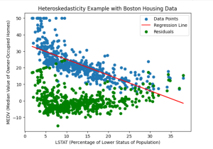
plt.title('Heteroskedasticity Example with Boston Housing Data')
plt.legend()
plt.show()
Here is how the plot would look like representing heteroskedasticity in green.

In the above code, a linear regression model is fit to the Boston housing dataset. The model is trained using the fit(X, y) method, where X represents the independent variable (lstat) and y represents the dependent variable (medv). Once the model is fitted, we predict the values of y using predict(X), resulting in y_predicted. We then calculate the residuals by subtracting the predicted values from the actual y values.
For analysing heteroskedasticity, we visualize the scatter plot of the data points, the regression line, and the residuals using matplotlib. The scatter plot displays the relationship between LSTAT and MEDV, with the regression line representing the estimated linear relationship. The residuals, shown as green points, provide insight into the presence and pattern of heteroskedasticity.
By examining the scatter plot and residuals, we can visually assess whether heteroskedasticity is present in the relationship between LSTAT and MEDV. You may note that the residuals exhibit a pattern where the spread varies systematically across the range of LSTAT values. Thus, it indicates the presence of heteroskedasticity.
Conclusion
Heteroskedasticity is a critical consideration in regression models. Failing to address heteroskedasticity can lead to biased estimates, unreliable hypothesis tests, and suboptimal predictions. In this blog, we learned the concept of heteroskedasticity and its implications through a real-world example using the Boston Housing dataset. By visually analyzing scatter plots and residuals, we demonstrated how heteroskedasticity can be detected and its effects understood. Armed with this knowledge, data scientists can employ techniques such as transformations, weighted least squares, robust regression, or generalized least squares to mitigate the impact of heteroskedasticity and build more reliable regression models. Understanding and addressing heteroskedasticity is crucial for extracting accurate insights, making informed decisions, and maximizing the potential of regression analysis.

Check out my latest book titled as First Principles Thinking: Building winning products using first principles thinking.
- Mathematics Topics for Machine Learning Beginners - July 6, 2025
- Questions to Ask When Thinking Like a Product Leader - July 3, 2025
- Three Approaches to Creating AI Agents: Code Examples - June 27, 2025
I found it very helpful. However the differences are not too understandable for me