When it comes to building a regression model, one comes across the question such as whether to train the regression model using DecisionTree Regressor algorithm or linear regression algorithm? The following is the key differences you need to know in order to decide which algorithm is the most suitable one, and, why and when one can use one over the other?
Linear vs Non-Linear Dataset: Which Algorithm to Use?
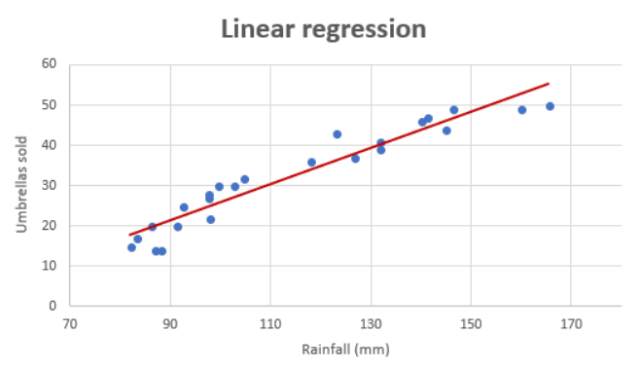
Linear regression algorithm can be used when there exists linear relationship between the response and predictor variables in the given data set. For two or three dimensional datasets, it is as easy as draw scatter plot and find about the said linear relationship. The following represents the linear relationship between number of umbrellas sold (response variable) vs rainfall in mm (predictor variable).
For multi-dimensional dataset, it is recommended to use dimensionality reduction algorithms such as principal component analysis (PCA) to find about appropriateness of using linear regression algorithm.
Decision tree regressor can be suitable for all kinds of dataset including cases where the relationship between the response and predictor variables is non-linear. Thus, if you found that the relationship in the datasets is non-linear, you can try with decision tree regression. Having said that, it comes with its own set of disadvantages including overfitting.
Prediction Output: Continuous vs Partially Continuous
The prediction of linear regression model is continuous in nature. This essentially means that each input will result in different output.
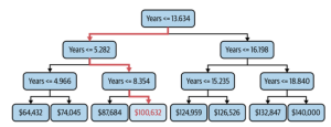
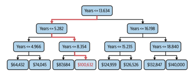
However, with decision tree regression, for a set of inputs, there might be just one output. Take a look at the following picture. It represents prediction of salary based on years of experience.
In the above decision tree (salary vs years of experience), you would note that for years’ values such as 9, 10, 11, 12, 13, the output will be $100,632. For years values such as 7 and 8, the value will be $87,684. So, you can notice that although the predicted value is continuous, it remains same for a set of inputs.
Parametric vs Non-parametric Model
Linear regression models are parametric in nature. This means that data is fit to a parametric mathematical equation consisting of one or more parameters. Decision tree regression models are non-parametric in nature. All that is needed to build a decision tree regressor is decision about which column or feature to choose for each node of the tree and what value to split the data on that node.
The very nature of parametric model makes it explanatory in nature (responsible AI). This is very useful in AI use cases which requires explanation for prediction made. For example, healthcare or finance related use cases. However, the catch is linear relationship present in dataset between predictor and response variables.
Python Implementations
The linear regression algorithm is implemented using LinearRegression class – sklearn.linear_model.LinearRegression. The following is simplistic implementation using this class.
import numpy as np
from sklearn.linear_model import LinearRegression
import matplotlib.pyplot as plt

# Example data
X = np.array([1, 2, 3, 4, 5]).reshape(-1, 1)  # Reshape for sklearn
y = np.array([2, 4, 5, 4, 5])

# Create and train the model
model = LinearRegression()
model.fit(X, y)

# Make predictions
X_test = np.array([6, 7]).reshape(-1, 1)
predictions = model.predict(X_test)

# Output the coefficients and intercept
print("Coefficient (slope):", model.coef_[0])
print("Intercept:", model.intercept_)
print("Predictions:", predictions)

# Plot the results
plt.scatter(X, y, color='blue', label='Actual Data')
plt.plot(X, model.predict(X), color='red', label='Fitted Line')
plt.scatter(X_test, predictions, color='green', label='Predictions')
plt.xlabel('X')
plt.ylabel('y')
plt.legend()
plt.show()
The following is the output for the above code:
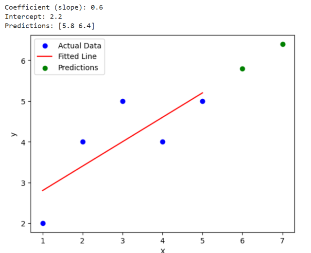
The DecisionTreeRegressor is implemented using DecisionTreeRegressor class – sklearn.tree.DecisionTreeRegressor.
import numpy as np
from sklearn.tree import DecisionTreeRegressor
import matplotlib.pyplot as plt

# Example data
X = np.array([1, 2, 3, 4, 5]).reshape(-1, 1)  # Reshape for sklearn
y = np.array([2, 4, 5, 4, 5])

# Create and train the model
model = DecisionTreeRegressor()
model.fit(X, y)

# Make predictions
X_test = np.array([6, 7]).reshape(-1, 1)
predictions = model.predict(X_test)

# Output the predictions
print("Predictions:", predictions)

# Plot the results
plt.scatter(X, y, color='blue', label='Actual Data')
X_range = np.linspace(X.min(), X.max(), 500).reshape(-1, 1)
y_range_pred = model.predict(X_range)
plt.plot(X_range, y_range_pred, color='red', label='Decision Tree Prediction')
plt.scatter(X_test, predictions, color='green', label='Test Predictions')
plt.xlabel('X')
plt.ylabel('y')
plt.legend()
plt.show()
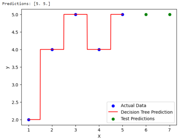
The following is how the output looks like:
- The Watermelon Effect: When Green Metrics Lie - January 25, 2026
- Coefficient of Variation in Regression Modelling: Example - November 9, 2025
- Chunking Strategies for RAG with Examples - November 2, 2025

I found it very helpful. However the differences are not too understandable for me