Last updated: 28th Nov, 2023
Understanding the difference between coefficient of variation (CV) and standard deviation (SD) is essential for statisticians and data scientists. While both concepts measure variability in a dataset, they are calculated differently and can be used in different scenarios for better understanding. Here, we will explore the coefficient of variation vs standard deviation differences to gain a better understanding of how to use them.
Coefficient of Variation vs Standard Deviation
Coefficient of Variation (CV) is a measure that is used to compare the amount of variation in a dataset relative to its mean value. It is calculated by taking the standard deviation divided by the mean, then multiplying by 100. At times, it is also termed as coefficient of standard deviation although many argue that this is not a standard term in statistics. Coefficient of variation can be interpreted as the percentage variation from the mean. This measure is useful for comparing the degree of variation from one data series to another, even if the means are drastically different. It is especially useful when comparing the degree of variation between datasets with different units or vastly different means.
Standard deviation (SD) is a measure of the amount of variation or dispersion in a set of values. It describes how far away any given sample or observation may be from the mean value found within that dataset or population. A low standard deviation means that the values tend to be close to the mean, while a high standard deviation means that the values are spread out over a wider range. When interpreting standard deviation, it’s important to consider whether it reflects normal distribution or not; if not, then other measures such as median should be considered instead. Additionally, since it only considers one variable at a time, it cannot be used for comparing two different datasets with different scales – this is where coefficient of variation comes in handy! Check out my related post – Standard Deviation of Population vs Sample.
Comparing two distributions as a function of how far the values lie from the mean in form of standard deviation provides greater insights by calculating Z-score. Z-scores measure the number of standard deviations that a point is away from the mean.
# Difference
The most significant difference between the coefficient of variation (CV) and standard deviation (SD) lies in their relative versus absolute measures of dispersion.
| Feature | Standard Deviation | Coefficient of Variation |
|---|---|---|
| Type of Measure | Absolute measure of dispersion | Relative measure of dispersion |
| Description | Provides the average distance of each data point from the mean | Expresses standard deviation as a percentage of the mean |
| Units | Expressed in the same units as the data | Dimensionless (percentage, no units) |
| Comparability | Best used for comparing variability within the same dataset | Allows for comparison across datasets with different units or means |
| Primary Application | Useful in understanding spread within a single dataset | Ideal for comparing variability across different datasets |
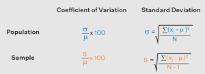
# Formula
The following is the formula of coefficient of variation and standard deviation across sample and population.

In the above formula of standard deviation and coefficient of variation, $\sigma$ represents standard deviation of population, s represents standard deviation of the sample, $\mu$ represents the mean, $x_i$ represents individual observation, N represents total number of observation.
# Python code examples
Here is the Python code for how to calculate coefficient of variation:
import numpy as np
# Define your dataset as an array
data = np.array([1, 2, 3, 4, 5])
# Calculate the mean of the data set
mean = np.mean(data)
# Calculate standard deviation
std_dev = np.std(data)
# Calculate coefficients of variation(CV)
cv = std_dev*100 / mean
# Print CV value
print('Coefficient of Variation (CV):', round(cv, 4))
Here is the python code for how to calculate the standard deviation:
import numpy as np
data = [10, 20, 30, 40]
stdev = np.std(data)
print("Standard Deviation is:", stdev)
# Examples
The coefficient of variation can be useful in comparison of standard deviations of data with different means. For example, if you were comparing salaries of two professions with vastly different average salaries, CV would allow you to make a comparison based on how much each salary varied from its respective mean. On the other hand, standard deviation would only help us learn about how much the salaries (from mean) vary in each of the profession.
Here are some real-life examples of usage of coefficient of variation:
- Coefficient of variation (CV) can be used to assess the risk associated with investments. A higher coefficient of variation value indicates a higher level of risk, as it indicates greater volatility and a wider range in the data. Let’s say there are two different stocks A and stocks B.
Stocks A price across 6 weeks are [15, 20, 12, 10, 18, 22]. The following will be mean, standard deviation and coefficient of variation:
CV = 26.34%
Mean = $16.17
Standard deviation = $4.26
The standard deviation of stock A is 26.34% of mean.
Stock B price across 6 weeks are [57, 68, 64, 71, 62, 72]. The following will be mean, standard deviation and coefficient of variation:
CV = 7.99%
Mean = $65.67
Standard deviation = $5.25
The standard deviation of stock B is 7.99% of mean.
With the standard deviation as the measure of risk, stock B is more risky over this period of time because it has a larger standard deviation ($5.25). However, the average price of stock B is almost four times as much as that of stock A. Relative to the amount invested in stock A, the standard deviation of $4.26 may not represent as much risk as the standard deviation of $5.25 for stock B, which has an average price of only $65.67. The coefficient of variation reveals the risk of a stock in terms of the size of standard deviation relative to the size of the mean (in percentage). Stock A has a coefficient of variation that is nearly three times as much as the coefficient of variation for stock B. Using coefficient of variation as a measure of risk indicates that stock A is riskier.
From investment perspective, stock A could indicate a higher potential reward, but also carries an increased possibility of losses. It is therefore important to consider the CV when evaluating any potential investment opportunities. - Assessing financial risk: Coefficient of variation can be used to evaluate how much financial risk a company is exposed to in comparison with the average amount for similar companies in its industry. This can help determine if the company has taken on too much risk or not.
- In the retail industry, coefficient of variation (CV) can be used to measure and compare the variability in sales across different stores or locations.
How & When to Use Coefficient of Variation vs Standard Deviation for driving decisions
Let’s consider an example to illustrate how the use of the coefficient of variation and standard deviation can drive decision making.
Suppose we have two classes of students, Class A and Class B, and we want to compare the variability of their test scores. Here are the test scores for each class:
Class A: 80, 85, 90, 92, 95
Class B: 70, 75, 80, 85, 90
As per the code below, the following comes out to be value of standard deviation and coefficient of variation:
Class A: SD = 5.72, CV = 6.92%
Class B: SD = 7.91, CV = 9.88%
import statistics
# Test scores for Class A and Class B
class_a_scores = [80, 85, 90, 92, 95]
class_b_scores = [70, 75, 80, 85, 90]
# Calculating Standard Deviation
class_a_sd = statistics.stdev(class_a_scores)
class_b_sd = statistics.stdev(class_b_scores)
# Calculating Coefficient of Variation
class_a_cv = (class_a_sd / statistics.mean(class_a_scores)) * 100
class_b_cv = (class_b_sd / statistics.mean(class_b_scores)) * 100
# Printing the results
print("Class A - Standard Deviation:", round(class_a_sd, 2))
print("Class B - Standard Deviation:", round(class_b_sd, 2))
print("Class A - Coefficient of Variation:", round(class_a_cv, 2))
print("Class B - Coefficient of Variation:", round(class_b_cv, 2))
The CV values indicate that the test scores in Class B have relatively higher variability compared to Class A. This comparison is possible because the coefficient of variation allows us to standardize the dispersion by taking into account the mean of each dataset.
Here is how the above coefficient of variation metrics help drive the decisions:
- Instructional Approaches: The higher variability in Class B’s test scores suggests that the students’ performance varies more widely within the class. This insight can prompt teachers and instructors to consider adopting differentiated instructional approaches. They may need to provide additional support and resources to address the diverse learning needs and ensure that all students have opportunities to succeed.
- Curriculum Adaptation: The wider variability in Class B may indicate that some students are struggling or not sufficiently challenged. This insight can drive decisions to adapt the curriculum, providing additional resources, enrichment activities, or targeted interventions for students who need extra support. It can help identify specific topics or skills where students require more attention and tailor instruction accordingly.
- Grouping and Differentiation: The greater variability in Class B may indicate a need for differentiated grouping strategies. Teachers can consider grouping students based on their performance levels, allowing for targeted instruction and support within smaller groups. This approach enables teachers to tailor the curriculum and instructional strategies to meet the diverse needs and abilities of students.
Frequently Asked Questions (FAQs)
The following are some of the most common frequently asked questions regarding standard deviation vs coefficient of variation:
- What’s the difference between variance and coefficient of variation?
- Variance and coefficient of variation are different statistical measures. Variance measures the spread of data points around the mean within a dataset, calculated as the average of the squared differences from the mean. It gives the dispersion’s magnitude but not relative to the mean. The coefficient of variation, on the other hand, is a normalized measure of dispersion, calculated as the standard deviation divided by the mean, often expressed as a percentage. This ratio allows comparison of variability across datasets with different units or scales, providing a relative sense of dispersion in relation to the mean.
- What’s coefficient of standard deviation?
- The term “coefficient of standard deviation” is not commonly recognized in statistics terminology. It might be a mistaken reference to either the standard deviation, which measures the spread of data points in a dataset, or the coefficient of variation, which is the ratio of the standard deviation to the mean, used to compare variability across different datasets.
- What is sample coefficient of variation formula?
- The sample coefficient of variation (CV) is calculated as the ratio of the sample standard deviation (s) to the sample mean, often expressed as a percentage. Note the usage of “sample”
Conclusion
To sum up, Coefficient of Variation and Standard Deviation are two different ways of measuring variability in datasets or populations. While both measures are useful for calculating variance, they differ in their applications – CV is best for making comparisons between datasets with different scales whereas SD should be used when dealing with just one variable at a time – and should always factor in normal distribution when interpreting results. Data scientists and statisticians should understand when each measure should be used depending on their goals so that they can get accurate results each time!

Check out my latest book titled as First Principles Thinking: Building winning products using first principles thinking.
- Mathematics Topics for Machine Learning Beginners - July 6, 2025
- Questions to Ask When Thinking Like a Product Leader - July 3, 2025
- Three Approaches to Creating AI Agents: Code Examples - June 27, 2025
I found it very helpful. However the differences are not too understandable for me