Autoregressive (AR) models, which are used for text generation tasks and time series forecasting, can be employed to predict future values predicated on previous observations. This blog post will provide the concepts of autoregressive (AR) models with Python code examples to demonstrate how you can implement an AR model for time-series forecasting. Note that time-series forecasting is one of the important areas of data science/machine learning. In subsequent blogs, we will take up the topic of how autoregressive models can be used as generative model for text generation tasks.
For beginners, time-series forecasting is the process of using a model to predict future values based on previously observed values. Time-series data is a sequence of data points, typically ordered in time. Forecasting models usually make predictions at regular intervals, such as hourly, daily, or weekly. Machine learning can be used to develop time-series forecasting models. This type of model is trained on past data and can be used to make predictions about future events. Time series forecasting is a valuable tool for businesses that can help them to make decisions about future production, staffing, and inventory levels. It can also be used to predict consumer demand and trends.
As mentioned above, autoregressive models can be utilized for text generation tasks, where the prediction of the next word depends on the words that have come before it. This sequential nature of the autoregressive models makes them particularly useful in fields like natural language processing.
Autoregressive (AR) Models concepts with Examples
Autoregressive (AR) modeling is one of the techniques used for time-series analysis. An autoregressive model is a time-series model that describes how a particular variable’s past values influence its current value. In other words, an AR model attempts to predict the next value in a series by incorporating the most recent past values and using them as input data. Autoregressive models are based on the idea that past events can help us predict future events. For example, if we know that the stock market has been going up for the past few days, we might expect it to continue going up in the future. Or, if we know that there has been a lot of rain lately, we might expect more rain in the future.
Autoregressive modeling is training a regression model on the value of the response variable itself. Autoregressive is made of the word, Auto and Regressive which represents the linear regression on itself (auto). In the context of time-series forecasting, autoregressive modeling will mean creating the model where the response variable Y will depend upon the previous values of Y at a pre-determined constant time lag. The time lag can be daily (or 2, 3, 4… days), weekly, monthly, etc. A great way to explain this would be that if I were predicting what the stock price will be at 12 pm tomorrow based on the stock price today, then my model might have an auto part where each day affects the next day’s value just like regular linear regression does but also has regressive features which mean there are different factors influencing changes over shorter spans such as days rather than weeks. AR models can be used to model anything that has some degree of autocorrelation which means that there is a correlation between observations at adjacent time steps. The most common use case for this type of modeling is with stock market prices where the price today (t) is highly correlated with the price one day ago (t-1).
[latex]Y_t = \beta_0 + \beta_1*Y_{t-1} + error_t[/latex]
In the above model, the value at the last time lag is taken. If the time lag is weekly, the [latex]Y_{t-1}[/latex] will represent the value of Y of the last week. Such AR models where the value of response variable of just one-time lag is taken are called AR models of the first model or AR (1) models. Let’s understand with the simple example of refrigerator sales. The ask is to forecast sales on a particular day in the future. And, the data we have is historical sales data of every day for last 3 years. AR model of 1st order with a time lag of 1 week will consider the refrigerator sale of last week.
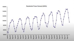
Let’s understand the AR model concept with another example and the following diagram.
The above diagram represents the residential power demand across different months from 2003 to 2010. The ask will be to use the data to forecast the power demand in the coming months. Taking time lag of 1 month, AR (1) model or AR model of 1st order will look like the following:
[latex]PowerDemand_t = \beta_0 + \beta_1*PowerDemandY_{t – 1} + error_t[/latex]
AR models have the parameter termed as p. The parameter p represents the previous values of p number of time lags when training the model. The AR model of 2nd order will have the value of the response variable at any particular time depending upon the values of the last two lags. Thus, AR (2) model will look like the following:
[latex]Y_t = \beta_0 + \beta_1*Y_{t-1} + \beta_2*Y_{t-2} + error_t[/latex]
Generalizing the above for p, the AR (p) model will look like the following:
[latex]Y_t = \beta_0 + \beta_1*Y_{t-1} + \beta_2*Y_{t-2} + … + \beta_p*Y_{t-p} + error_t[/latex]
Alternatives Methods to AR Models
Here are some of the alternative time-series forecasting methods to the AR modeling technique:
- MA (Moving average)
- ARMA (Autoregressive moving average)
- ARIMA (Autoregressive integrated moving average)
- SARIMA (Seasonal autoregressive integrated moving average)
- VAR (Vector autoregression)
- VARMA (Vector autoregression moving average)
- SES (Simple exponential smoothing)
We will discuss the above time-series modeling technique in upcoming blog posts.
Python Code Example for AR Model
We will use statsmodels.tsa package to load ar_model.AR class which is used to train the univariate autoregressive (AR) model of order p. Note that statsmodels.tsa contains model classes and functions that are useful for time series analysis. Basic models include univariate autoregressive models (AR), vector autoregressive models (VAR), and univariate autoregressive moving average models (ARMA). The following are some of the key steps which needed to be done for training the AR model:
- Plot the time-series
- Check the stationarity
- Determine the parameter p or order of the AR model
- Train the model
Here is the Python code example for the AR model trained using statsmodels.tsa.ar_model.AutoReg class.
import pandas as pd
import numpy as np
import matplotlib.pyplot as plt
#
# Load AutoReg class from statsmodels.tsa.ar_model module
#
from statsmodels.tsa.ar_model import AutoReg
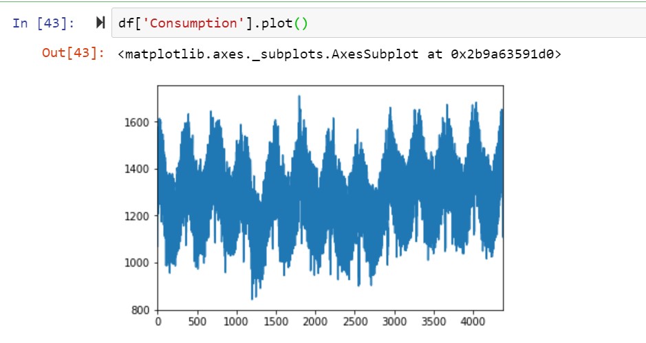
# Load and plot the time-series data
#
url='https://raw.githubusercontent.com/jenfly/opsd/master/opsd_germany_daily.csv'
df = pd.read_csv(url,sep=",")
df['Consumption'].plot()
Here is how the time-series plot will look like.
Before going ahead and training the AR model, the following will be needed to be found:
- Stationarity of the time-series data: The stationarity of the data can be found using adfuller class of statsmodels.tsa.stattools module. The value of p-value is used to determine whether there is stationarity. If the value is less than 0.05, the stationarity exists.
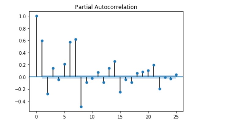
- Order of AR model to be trained: The order of AR model is determined by checking the partial autocorrelation plot. The plot_pacf method of statsmodels.graphics.tsaplots is used to plot.
The following code is used to check the stationarity and order of the AR model.
#
# Check for stationarity of the time-series data
# We will look for p-value. In case, p-value is less than 0.05, the time series
# data can said to have stationarity
#
from statsmodels.tsa.stattools import adfuller
#
# Run the test
#
df_stationarityTest = adfuller(df['Consumption'], autolag='AIC')
#
# Check the value of p-value
#
print("P-value: ", df_stationarityTest[1])
#
# Next step is to find the order of AR model to be trained
# for this, we will plot partial autocorrelation plot to assess
# the direct effect of past data on future data
#
from statsmodels.graphics.tsaplots import plot_pacf
pacf = plot_pacf(df['Consumption'], lags=25)
The following plot can be used to determine the order of AR model. You may note that a correlation value up to order 8 is high enough. Thus, we will train the AR model of order 8.
The next step is to train the model. Here is the code which can be used to train the model.
#
# Create training and test data
#
train_data = df['Consumption'][:len(df)-100]
test_data = df['Consumption'][len(df)-100:]
#
# Instantiate and fit the AR model with training data
#
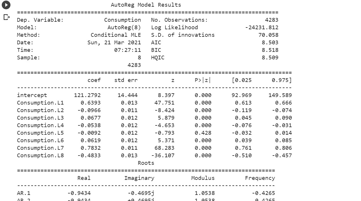
ar_model = AutoReg(train_data, lags=8).fit()
#
# Print Summary
#
print(ar_model.summary())
Here is how the summary will look like:
Once the model is trained, the final step is to make the predictions and evaluate the predictions against the test data. This is the code that can be used to do the same.
#
# Make the predictions
#
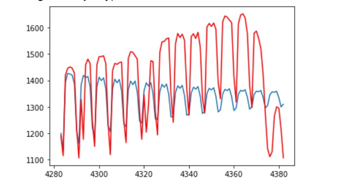
pred = ar_model.predict(start=len(train_data), end=(len(df)-1), dynamic=False)
#
# Plot the prediction vs test data
#
from matplotlib import pyplot
pyplot.plot(pred)
pyplot.plot(test_data, color='red')
This is how the plot will look like:
Learning References
Here are some good learning references for auto-regressive models:
Autoregressive models are powerful tools in the data scientist’s toolbox for understanding how one variable may predict another. The examples we’ve provided should give you a starting point to implement autoregressive modeling into your own work or research projects, but if this is all new to you, reach out for help!

Check out my latest book titled as First Principles Thinking: Building winning products using first principles thinking.
- Questions to Ask When Thinking Like a Product Leader - July 3, 2025
- Three Approaches to Creating AI Agents: Code Examples - June 27, 2025
- What is Embodied AI? Explained with Examples - May 11, 2025
I found it very helpful. However the differences are not too understandable for me