In this post, you will learn about validation curves with Python Sklearn example. You will learn about how validation curves can help diagnose or assess your machine learning models in relation to underfitting and overfitting. On the similar topic, I recommend you reading one of the previous post on assessing overfitting and underfitting titled Learning curves explained with Python Sklearn example.
The following gets covered in this post:
- Why validation curves?
- Python Sklearn example for validation curves
Why Validation Curves?
As like learning curve, the validation curve also helps in diagnozing the model bias vs variance. The validation curve plot helps in selecting most appropriate model parameters (hyper-parameters). Unlike learning curve, the validation curves helps in assessing the model bias-variance issue (underfitting vs overfitting problem) against the model parameters. In the example shown in the next section, the model training and test scores have been plotted against the inverse regularization parameters C for estimator LogisticRegression.
Python Sklearn Example for Validation Curves
In this section, you will learn about Python Sklearn code which can be used to create the validation curve. Sklearn IRIS dataset is used for illustration purpose. Pay attention to some of the following:
- Sklearn Pipeline is used for training the model. As part of pipeline, StandardScaler is used for standardization and LogisticRegression is used as an estimator.
- StraifiedKFold cross-validation technique is used to measure training and test scores across 10 folds
- Validation curve represents model scores (accuracy) for training and test data against the inverse regularization parameter C. For that purpose, it takes two specific input parameters such as param_name (logisticregression__C and param_range (different values of C)
import pandas as pd
import numpy as np
import matplotlib.pyplot as plt
import seaborn as sns
from sklearn import datasets
from sklearn.model_selection import train_test_split
from sklearn.model_selection import validation_curve
from sklearn.preprocessing import StandardScaler
from sklearn.pipeline import make_pipeline
from sklearn.linear_model import LogisticRegression
#
# IRIS Dataset is loaded
#
iris = datasets.load_iris()
df = pd.DataFrame(iris.data)
df.columns = ['sepal_length', 'sepal_width', 'petal_length', 'petal_width']
df['species'] = iris.target
#
# Create training and test split
#
X_train, X_test, y_train, y_test = train_test_split(df.iloc[:, :-1], df.iloc[:, -1], test_size=0.3, random_state=1,
stratify=df.iloc[:, -1])
#
# Create the pipeline having steps for standardization and estimator as LogisticRegression
#
pipeline = make_pipeline(StandardScaler(), LogisticRegression(solver='lbfgs', penalty='l2', max_iter=10000, random_state=1))
#
# Get Training and test scores using validation curve method
# Pay attention to the parameter values range set as param_range
#
param_range = [0.001, 0.05, 0.1, 0.5, 1.0, 10.0]
train_scores, test_scores = validation_curve(estimator=pipeline,
                                             X=X_train, y=y_train,
                                             cv=10,
param_name='logisticregression__C', param_range=param_range)
#
# Find the mean of training and test scores out of 10-fod StratifiedKFold cross validation run as part fo execution of validation curve
#
train_mean = np.mean(train_scores, axis=1)
test_mean = np.mean(test_scores, axis=1)
#
# Plot the model scores (accuracy) against the paramater range
#
plt.plot(param_range, train_mean,
         marker='o', markersize=5,
         color='blue', label='Training Accuracy')
plt.plot(param_range, test_mean,
         marker='o', markersize=5,
         color='green', label='Validation Accuracy')
plt.xlabel('Parameter C')
plt.ylabel('Accuracy')
plt.grid()
plt.show()
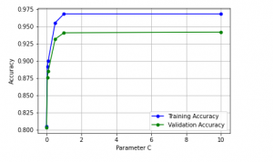
Here is how the validation curve plot representing model scores (accuracy) against regularization parameter C will look like:
Here is some of the observations from the above plot:
- For lower value of C (greater strength of regularization), the model tends to underfits.
- For larger value of C (lesser strength of regularization), the model tends to overfits. This can be evident by greater gap between model scores between training data and test data with model scores for training much higher than test data
- The sweet spot looks to appear between the C value of 0.05 and 0.5.
Conclusions
Here is the summary of what you learned in this post:
- Use validation curve for diagnozing model bias vs variance vis-a-vis the model parameters
- For some values of model parameters, model may underfit while for other values, model may overfit. It is important to identify the sweet spot.
- As like learning curve, Sklearn pipeline is used for creating the validation curve.
- Like learning curve, validation curve helps in assessing or diagnosing the model bias – variance issue. This is the similarity between learning and validation curve.
- Unlike learning curve, validation curve plots the model scores against model parameters. Recall that learning curve plots model scores against the training sample sizes. This the key difference between learning and validation curve.
- Sklearn.model_selection validation_curve method can be used for calculating training and test scores from training and test data.

Check out my latest book titled as First Principles Thinking: Building winning products using first principles thinking.
- Mathematics Topics for Machine Learning Beginners - July 6, 2025
- Questions to Ask When Thinking Like a Product Leader - July 3, 2025
- Three Approaches to Creating AI Agents: Code Examples - June 27, 2025
I found it very helpful. However the differences are not too understandable for me