Understanding the differences between the t-distribution and the normal distribution is crucial for anyone delving into the world of statistics, whether they’re students, professionals in research, or data enthusiasts trying to make sense of the world through numbers. But why should one care about the distinction between these two statistical distributions? The answer lies in the heart of hypothesis testing, confidence interval estimation, and predictive modeling.
When faced with a set of data, choosing the correct distribution to describe it can greatly influence the accuracy of your conclusions. The normal distribution is often the default assumption due to its simplicity and the central limit theorem, which states that the means of samples from a population will tend to follow a normal distribution, regardless of the shape of the population distribution. However, this assumption holds true only when dealing with large sample sizes.
Enter the t-distribution – a probability distribution which is used when we are working with small sample sizes or when the population variance is unknown. The t-distribution accounts for the extra uncertainty that comes with these conditions. By understanding the nuances between the t-distribution and the normal distribution, analysts can avoid missteps in data analysis that could lead to incorrect inferences about their data.
In this blog, we will dissect the t-distribution and the normal distribution, pinpoint their differences, and walk through examples that will help clarify when and why to use one over the other. Let’s dive in and unravel the intricacies of these fundamental distributions in the world of statistics.
t-distribution explained with Examples
Much like its well-known counterpart, the normal distribution, the t-distribution curve, as well, is a continuous and symmetrical curve. The t-distribution’s unique feature is that its precise shape is not fixed; rather, the shape of the probability distribution plot changes based on the degrees of freedom associated with the sample at hand. These degrees of freedom refer to the number of values in a calculation that are free to vary, and in the realm of the t-distribution, they’re intrinsically linked to sample size. To put it simply, as we collect more data, the degrees of freedom increase. This is akin to having a larger canvas to paint a picture—the more space you have, the more detail you can potentially add.
Consider a real-world scenario such as a startup trying to gauge the average satisfaction level of its service through customer feedback. With only a handful of customers, the startup must rely on the t-distribution, as every single response carries significant weight and impacts the overall picture of customer satisfaction. Each additional survey completed offers more freedom to the analysis, gradually shaping the t-distribution’s curve.
The following plots represent t-distribution for different degrees of freedom.
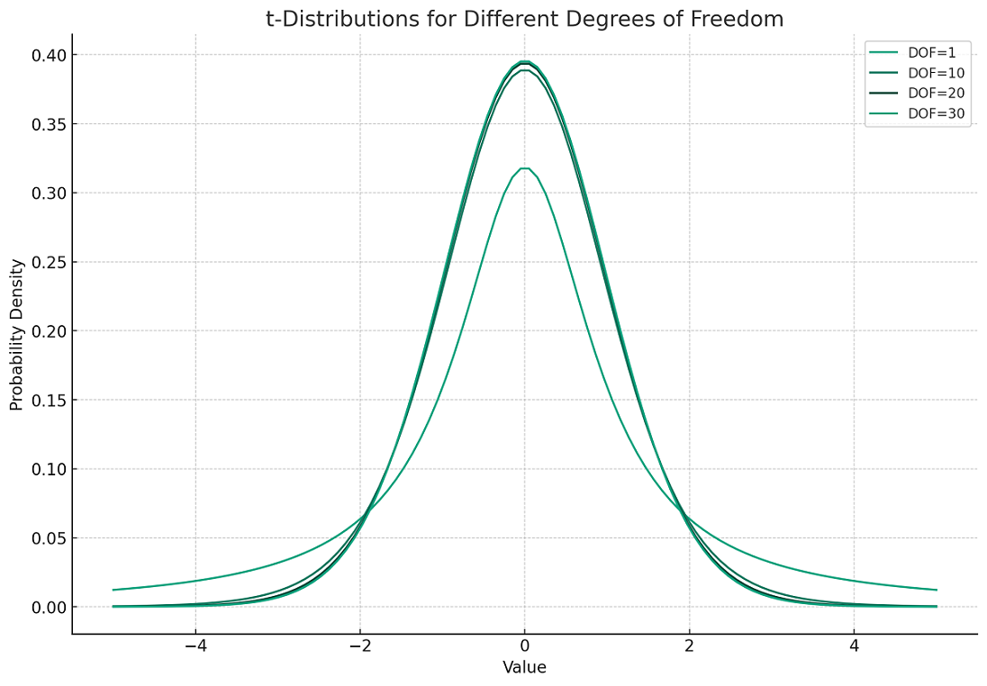
Here are the plots for the t-distributions with degrees of freedom 1, 10, 20, and 30. As you can see:
- With 1 degree of freedom (DOF=1), the t-distribution is much more spread out with heavier tails, which means there’s a higher probability of values further from the mean.
- As the degrees of freedom increase, the t-distribution starts to look more like the standard normal distribution; it becomes less spread with thinner tails.
- By the time we reach 30 degrees of freedom (DOF=30), the t-distribution is very close to the normal distribution in appearance, indicating that the extra uncertainty accounted for in smaller samples is becoming less significant.
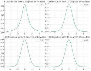
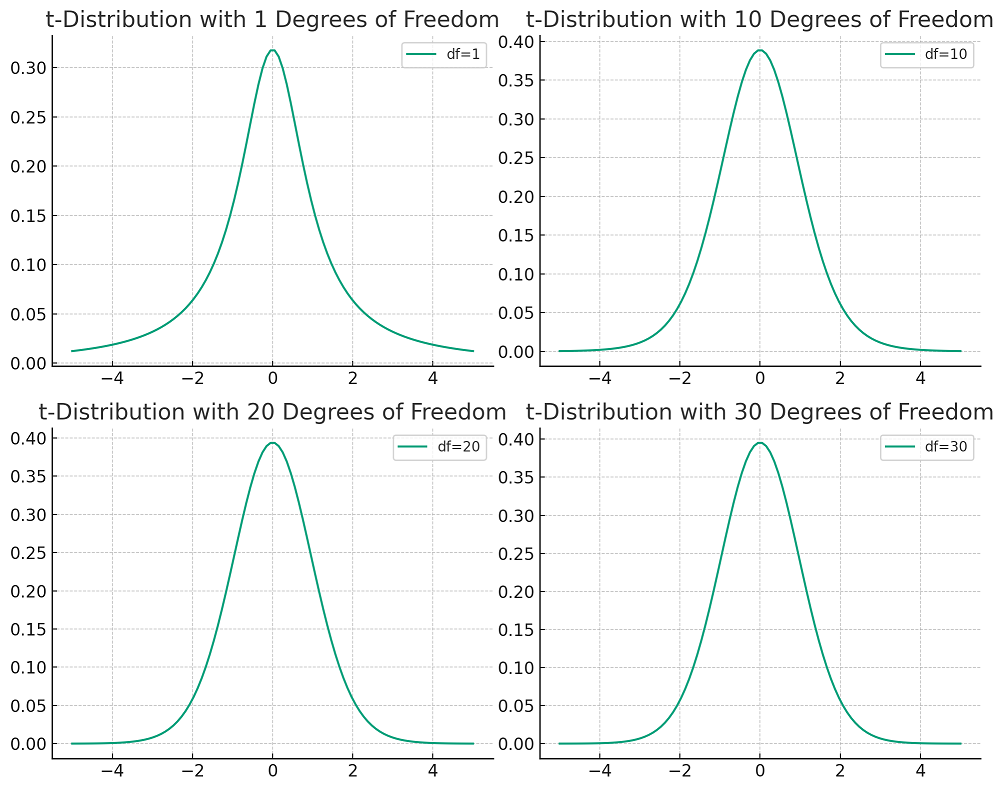
The following is grid view for the t-distribution plots related to above example.
The t-distribution becomes particularly valuable in two key scenarios. First, when researchers are working with small sample sizes—think of a scientist analyzing the effects of a new medication with only a limited number of trial subjects. With such a small group, any measurement is precious, and the t-distribution provides a more accurate reflection of the uncertainty in the results than the normal distribution would.
Secondly, when the population’s standard deviation—an indicator of how spread out the data is—is unknown, the t-distribution comes to the rescue. This is often the case in the early stages of market research, where companies are trying to understand consumer behavior for a new product. Without historical data, the standard deviation of the population is a mystery, leaving researchers to work with what they have: the sample’s standard deviation. When we draw samples from a normally distributed population and we don’t know the population standard deviation, the distribution of sample means for some variable x drawn from this population can be described by the formula
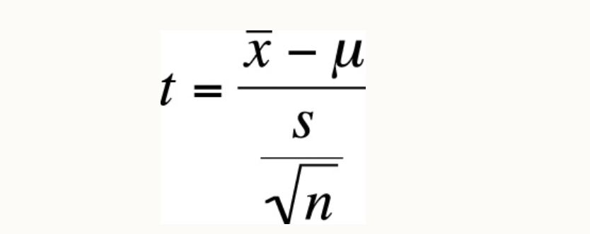
In the above formula, t represents t-statistics, s represents the sample standard deviation, n represents the sample size, mu represents the population mean and x-bar represents the sample mean. This formula is similar to the formula for the Z-statistic except for one difference; for the t-statistic, we use the sample standard deviation, whereas for the Z-statistic, we use the population standard deviation.
Normal Distribution explained with Examples
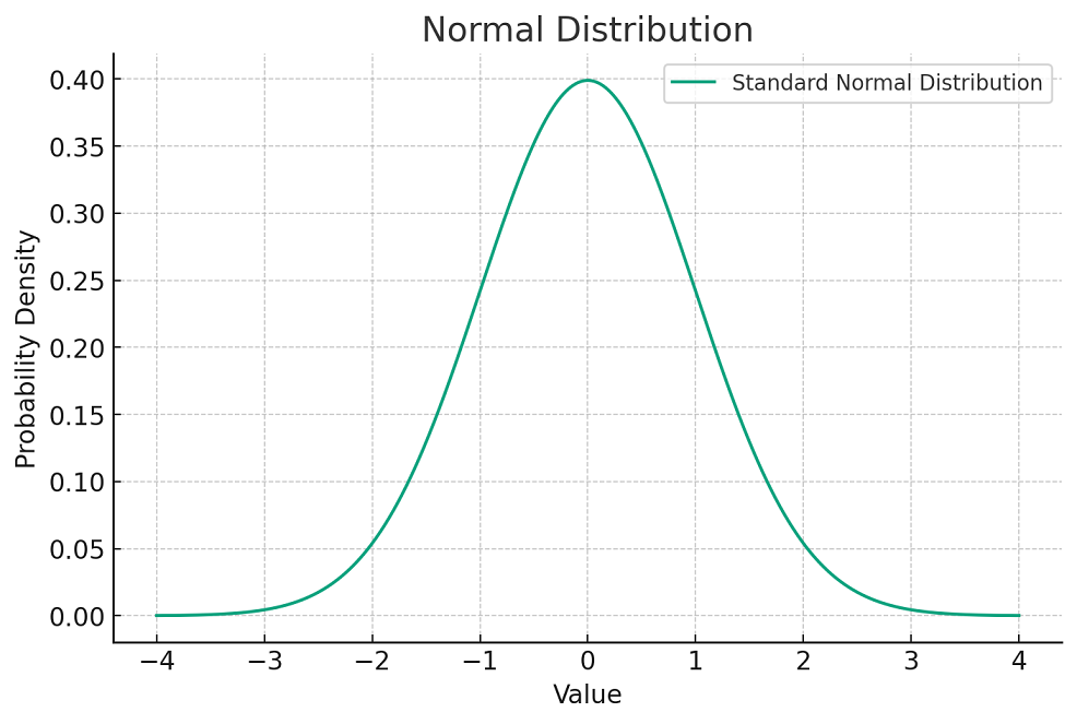
A normal distribution, also known as a Gaussian distribution, is a probability distribution that is symmetric about the mean, showing that data near the mean are more frequent in occurrence than data far from the mean. In graph form, the normal distribution will appear as a bell curve. Here is a plot of the standard normal distribution, which has a mean (μ) of 0 and a standard deviation (σ) of 1. The curve is symmetric about the mean and has a bell-shaped pattern, which is characteristic of a normal distribution. The peak of the curve represents the mean and the spread of the curve is determined by the standard deviation.
Here are the plots of three different normal distributions, each with distinct means (μ) and standard deviations (σ):
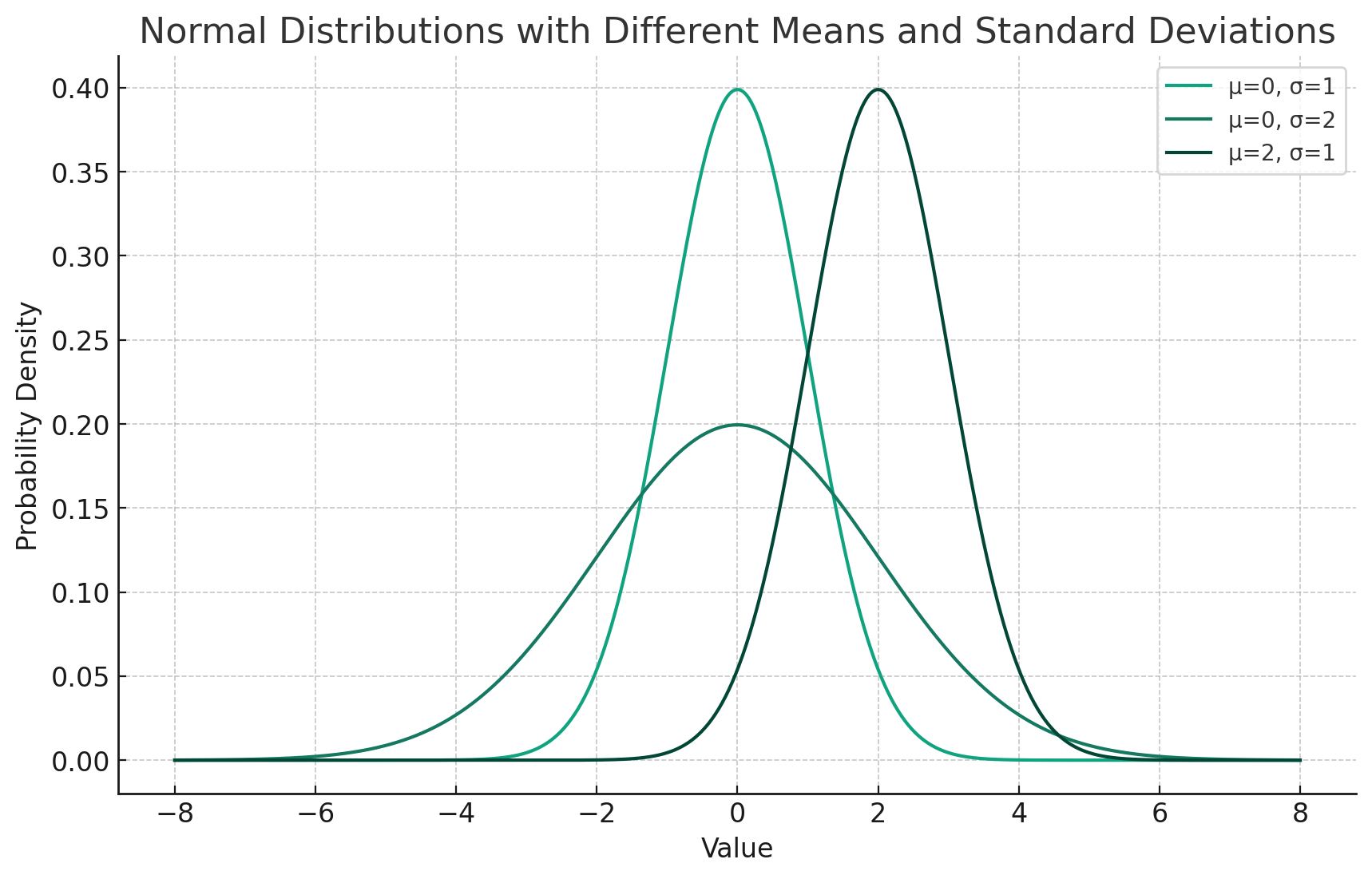
- The first distribution has a mean of 0 and a standard deviation of 1. It is the standard normal distribution.
- The second distribution also has a mean of 0 but a larger standard deviation of 2, making it flatter and wider, indicating more dispersion around the mean.
- The third distribution has a mean of 2 and a standard deviation of 1, which means it is centered around 2 on the x-axis but has the same degree of spread as the standard normal distribution.
The area under each curve represents the total probability of all outcomes and is equal to 1 for all three distributions. The difference in shape between these curves illustrates how changing the mean and standard deviation parameters can shift and scale the normal distribution.
Mathematically, the normal distribution is defined by two parameters: the mean (μ), which determines the center of the distribution, and the standard deviation (σ), which determines the width of the distribution. The mean is the point at which the curve is centered, and the standard deviation is a measure of the dispersion or spread of the distribution. The further away from the mean, the lower the curve.
The formula for the probability density function (PDF) of the normal distribution is:
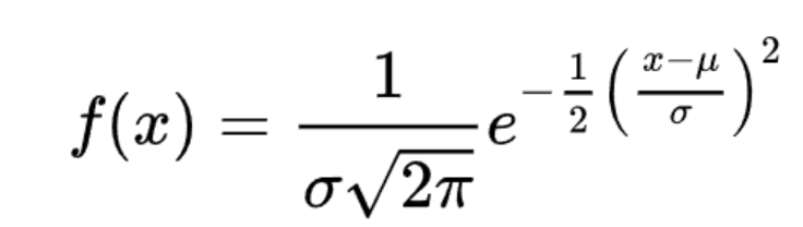
This function indicates the probability that a random variable that follows a normal distribution takes on the value x.
A key property of the normal distribution is that the area under the curve corresponds to the probability of occurrence and the total area under the curve integrates to 1.
Differences between t-distribution & Normal Distribution
The t-distribution and the normal distribution are both probability distributions that are used to describe the behavior of data in different situations. Here are some of the key differences between them:
- Shape:
- Normal Distribution: It has a bell-shaped curve and is symmetric around the mean. The shape of the normal distribution is the same regardless of the mean or standard deviation.
- T-distribution: Similar to the normal distribution in shape but has heavier tails. The t-distribution becomes wider and more variable as the sample size decreases, which is reflected in its degrees of freedom.
- Degrees of Freedom:
- Normal Distribution: It does not depend on the degrees of freedom. The normal distribution is based on populations with a known variance or large sample sizes where the sample variance is a good approximation of the population variance.
- T-distribution: The shape of the t-distribution varies with the degrees of freedom. Degrees of freedom typically correlate with the sample size (n – 1 for a single sample).
- Sample Size:
- Normal Distribution: It is used when dealing with large sample sizes (typically n > 30) or when the population variance is known.
- T-distribution: It is particularly useful for small sample sizes (typically n < 30) or when the population variance is unknown.
- Tail Probability:
- Normal Distribution: Less probability in the tails; it assumes that extreme values are less likely to occur.
- T-distribution: More probability in the tails; it accounts for the greater variability expected with smaller samples and unknown population standard deviation, thus providing more conservative estimates.
- Usage in Hypothesis Testing:
- Normal Distribution: Used in z-tests when the standard deviation of the population is known or the sample size is large.
- T-distribution: Used in t-tests which are applied when the standard deviation of the population is unknown and the sample size is small.
- Convergence:
- T-distribution: As the sample size increases (and thus the degrees of freedom), the t-distribution approaches the normal distribution. In the limit, as degrees of freedom go to infinity, the t-distribution becomes identical to the normal distribution.
- Standard Error:
- Normal Distribution: The standard error is based on the population standard deviation.
- T-distribution: The standard error is based on the sample standard deviation, which includes the correction factor of the square root of the degrees of freedom (n – 1).

Check out my latest book titled as First Principles Thinking: Building winning products using first principles thinking.
- Mathematics Topics for Machine Learning Beginners - July 6, 2025
- Questions to Ask When Thinking Like a Product Leader - July 3, 2025
- Three Approaches to Creating AI Agents: Code Examples - June 27, 2025
I found it very helpful. However the differences are not too understandable for me