
In the world of data science, understanding the relationship between variables is crucial for making informed decisions or building accurate machine learning models. Correlation is a fundamental statistical concept that measures the strength and direction of the relationship between two variables. However, without the right tools and knowledge, calculating correlation coefficients and p-values can be a daunting task for data scientists. This can lead to suboptimal decision-making, inaccurate predictions, and wasted time and resources.
In this post, we will discuss what Pearson’s r represents, how it works mathematically (formula), its interpretation, statistical significance, and importance for making decisions in real-world applications such as business forecasting or medical diagnosis. We will also explore some examples of using Pearson’s r (correlation coefficient) and p-value (used for statistical significance) with real data sets so you can see how this powerful statistic works in action. We will learn to use Python’s scipy.stats pearsonr method which is a simple and effective way to calculate the correlation coefficient and p-value between two variables. As a data scientist, it is very important to understand Pearson’s r and its implications for making decisions based on data.
What is Pearson Correlation Coefficient?
Pearson correlation coefficient is a statistical measure that describes the linear relationship between two variables. It is typically represented by the symbol ‘r’. Pearson correlation coefficient can take on values from -1 to +1 and it is used to determine how closely two variables are related. It measures the strength of their linear relationship, which means that it indicates whether one variable increases or decreases as the other variable increases or decreases. A Pearson correlation coefficient of 1 indicates a perfect positive (direct) linear relationship, while a Pearson correlation coefficient of -1 indicates a perfect negative (inverse) linear relationship. Furthermore, when Pearson’s r is 0 there is no linear relationship between the two variables.
It’s important to note that correlation does not imply causation. A significant Pearson’s r value indicates a linear association, but it doesn’t mean that one variable causes the other. Other factors, known as confounding variables, may influence this relationship. Additionally, Pearson’s r only measures linear relationships. If the relationship is non-linear, other statistical methods may be more appropriate to describe the association. A study finds a significant positive Pearson correlation coefficient () between monthly ice cream sales and the number of drowning incidents. The data show that as ice cream sales increase, the number of drowning incidents also increases. If we mistakenly infer causation from this correlation, we might conclude that eating ice cream leads to an increased risk of drowning.
The increase in both ice cream sales and drowning incidents might both be caused by a third variable (confounding variable): the temperature or season (i.e., summer). During summer months, temperatures are higher, which leads to more people buying ice cream. Simultaneously, more people are likely to engage in swimming activities, which increases the risk of drowning incidents. Temperature acts as a confounding variable that is associated with both ice cream sales and drowning incidents.
Pearson Correlation Coefficient vs Plots
The following plots represent linear relationship vis-a-vis different values of Pearson correlation coefficient.

The following is the explanation for the above plots:
-
Direct Linear Relationship ( close to +1): The first plot shows a clear upward trend, indicating that as increases, also increases. The points are closely aligned around a straight line, suggesting a strong positive linear relationship. The Pearson Correlation Coefficient for such a dataset would be close to +1, implying that the variables move together in the same direction.
-
No Linear Relationship ( close to 0): The second plot shows a scatter of points with no apparent pattern. There is no discernible slope, and the points do not align around any line. This randomness suggests that there is no linear relationship between and . In such a case, the Pearson Correlation Coefficient would be close to 0, indicating no linear correlation between the variables.
-
Inverse Linear Relationship ( close to -1): The third plot shows a clear downward trend, indicating that as increases, decreases. The points are closely aligned around a straight line, but this time the line slopes downwards, suggesting a strong negative linear relationship. The Pearson Correlation Coefficient for such a dataset would be close to -1, implying that the variables move in opposite directions.
Pearson Correlation Coefficient – Different Values vs Strength of Relationship
When assessing the linear relationship between two variables using correlation analysis, the magnitude of the correlation coefficient (ignoring the sign) provides insight into the strength of the relationship. Here’s a more detailed guide to interpreting the absolute value of the correlation coefficient:
-
: This represents a perfect correlation, indicating that for every change in one variable, there is a predictable and exact corresponding change in the other variable. In a graph, the data points would lie exactly on a straight line, either upwards or downwards, depending on the sign.
-
: When the correlation coefficient approaches this value, it is considered a strong correlation. This suggests a high degree of predictability in the relationship, where changes in one variable are closely followed by changes in the other, though not perfectly.
-
: This value signifies a moderate correlation. The relationship between the variables is evident and can be described as substantial, but there are other factors and variability influencing the relationship.
-
: This is indicative of a weak correlation, where there is a slight, possibly inconsistent association between the variables. The predictability is low, and while there may be a relationship, it is not strong and could be easily influenced by other variables.
-
: A zero or close to zero correlation coefficient means there is no linear correlation between the variables. There’s no predictable association that can be discerned from the data; any relationship is likely due to chance or randomness.
Pearson Correlation Coefficient – Real-world Examples
Pearson correlation coefficient can be used to examine relationships between variables in a variety of real-world applications such as some of the following:
- In medicine, Pearson’s r can be used to measure the strength of the relationship between patient age and cholesterol levels.
- In finance, Pearson’s r can be used to measure the strength of the relationship between stock prices and earnings per share.
- In business forecasting, Pearson’s r can be used to measure the strength of the relationship between sales and marketing efforts.
- In lifestyle research, Pearson’s r can be used to measure the strength of the relationship between exercise habits and obesity rates.
- Another example is measuring correlation between customer loyalty against customer satisfaction levels and ascertain whether customers who report higher levels of satisfaction also demonstrate higher levels of loyalty or vice versa. Another example could include studying height against weight wherein one might use Pearson’s correlation coefficient to measure if taller individuals tend to weigh more than their shorter counterparts on average or if there is no obvious connection present at all between height and weight when considering real-world data sets.
Pearson’s correlation coefficient has implications for hypothesis testing as well as other decision-making processes. By measuring the strength of a linear relationship between two variables, researchers can make informed decisions based on their findings which can help guide future research studies or inform corporate policies and practices. Pearson’s correlation coefficient also provides a basis for making predictions about future outcomes when given certain inputs or conditions–which is incredibly valuable in various business settings where predicting customer behavior or market trends is critical for success.
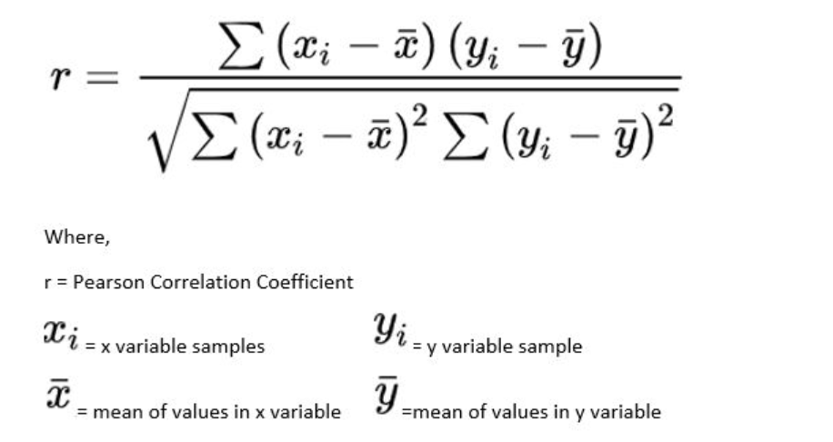
Pearson Correlation Coefficient – Formula
The Pearson Correlation Coefficient formula is given as the following:
Pearson Correlation Coefficients should not be taken as definitive proof that there is a relationship between two variables; rather they should only serve as indicators for further investigation which can then lead to more conclusive results regarding such relationships. In addition, Pearson Correlation Coefficients are considered reliable only when sample sizes are large enough and data points are normally distributed; if these conditions are not met then other statistical tests may be necessary in order to determine the significance of any indicated correlations.
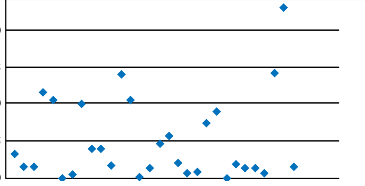
Scatterplots & Pearson Correlation Coefficient
Scatterplots are a powerful way of visualizing data and relationships between two variables.
They are graphs that display data points in which the values for two variables are plotted against each other. The x-axis usually displays one variable, and the y-axis displays the other variable. Each point on a scatter plot represents one data set composed of the independent and dependent variables being studied; when plotted in relation to each other, these points form clusters or patterns which allow us to analyze the strength and direction of the relationship between these variables.
When plotting scatter plots, Pearson’s correlation coefficient can be used to determine how closely related two variables are to each other by measuring the degree of association between them.
Pearson’s correlation coefficient is calculated using the formula:
r = ∑(x – x̅)(y – y̅) / √∑(x – x̅)²∑ (y – y̅)²
where x̅ and y̅ represent mean values for the respective x and y values.
By examining how closely points cluster together on a scatter plot, one can measure both linearity and strength in order to determine Pearson’s correlation coefficient value. The picture below represents correlation coefficient in three different scatter plots.
The picture below might represent a very high correlation coefficient closer to 1.

The picture below might represent decently high correlation coefficient closer to 0.5.

The picture below might represent a very low correlation coefficient closer to 0.
Pearson Correlation Coefficient Examples
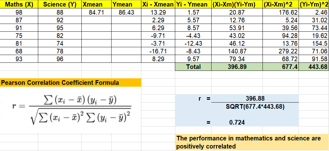
This example will illustrate how to use Pearson correlation coefficient (PCC) to determine the correlation between two continuous variables. In the example below, the marks of mathematics and science for a class of students in a school are considered for evaluating correlation. Based on the value of the PCC, data scientists can identify linear relationships between these two variables, providing invaluable insights about the data. Note the usage of PCC formula defined in earlier section.
Statistical Significance of Pearson Correlation Coefficient
In order to determine whether any given Pearson correlation coefficient has a statistically significant result or not, we will need to go through the following steps:
- Determine null & alternate hypothesis: The null hypothesis can be stated that there is no relationship between the two variables (r = 0) while the alternate hypothesis is that there is a relationship (r != 0).
- Determine statistics for hypothesis testing: We will calculate t-statistics and perform t-test with (n-2) degree of freedom
- Determine level of significance: The level of significance chosen is 0.05
- Calculate & compare t-statistics with critical value: We will test the significance by evaluating t-statistics and comparing it with critical value read from t-distribution table at 0.05 significance level. If the t-statistics value is greater than the critical value at 0.05, the null hypothesis can be rejected. This would mean that there is enough evidence to support the alternate hypothesis that there is some relationship between two variables.
The following is the formula for calculating the value of t-statistics for determining statistical significance of Pearson correlation coefficient:
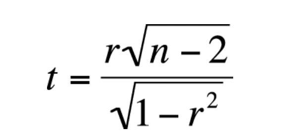
In the above formula, r is correlation coefficient value and n is sample size. In the example given in earlier section, the t-value will come out to be based on the following calculation. The value of n = 7 and value of r = 0.724.
$$ t = \frac{0.724\sqrt(7-2)}{\sqrt(1 – 0.724^2)} $$
$$t = 2.347 $$
One can also calculate p-value and compare it with 0.05 significance level. If p-value is less than 0.05, the Pearson correlation coefficient can be considered to be statistically significant and the null hypothesis rejected in favor of the alternate hypothesis. The degree of freedom = (N-2).
In above example, degree of freedom = (7-2) = 5.
Thus, p-value by looking at the t-distribution table for a two-tailed test with t-value as 2.347, df = 5 comes out to be 0.0658. Thus, at a 0.05 level of significance, we don’t have enough evidence to reject the null hypothesis (no relationship between the marks). Thus, based on given evidence, one can conclude that there is a statistical evidence that the linear variables such as marks of maths and science are not strongly correlated.
Recall that a P-value is a statistic that tells us how likely an observed result is due to chance alone. If a Pearson Correlation Coefficient has an associated P-value below 0.05, then it can be considered statistically significant. This means that the Pearson Correlation Coefficient is unlikely to have occurred by chance and thus supports the hypothesis that there is indeed some kind of relationship between the two variables being studied.
Calculating Correlation Coefficient & P-value using PearsonR
Here is the Python code for calculating the correlation coefficient and p-value. The data used in the code below is NPX & PeptideAbundance which can be accessed from Kaggle competition (Parkinson disease prediction) . NPX (Normalized protein expression) is the frequency of the protein’s occurrence in the sample. PeptideAbundance is the frequency of the amino acid in the sample
import pandas as pd
import numpy as np
from scipy.stats import pearsonr

# Read in data from CSV file
df = pd.read_csv('data.csv')

# Drop rows with NaN or Inf values
df = df.replace([np.inf, -np.inf], np.nan).dropna()

# Calculate correlation coefficient
corr, pval = pearsonr(df['NPX'], df['PeptideAbundance'])

# Print results
if pval < 0.05:
    print(f"The correlation coefficient between NPX and PeptideAbundance is {corr:.3f}, which is significant (p = {pval:.3f}).")
else:
    print(f"The correlation coefficient between NPX and PeptideAbundance is {corr:.3f}, which is not significant (p = {pval:.3f}).")
If the p-value is less than 0.05, we reject the null hypothesis and conclude that there is a significant correlation between the two variables. Otherwise, we fail to reject the null hypothesis, and we conclude that there is no significant correlation.
In the above code, the correlation coefficient and the p-value is printed. If the p-value is less than 0.05, it is printed that the correlation is significant; otherwise, it gets printed that the correlation is not significant.
Conclusion
In conclusion, Pearson correlation coefficient is a powerful tool that allows for measuring the strength of linear relationships between two variables. It has implications for decision-making processes and research studies as well as real-world applications such as medicine, finance, business forecasting and lifestyle research. Pearson’s correlation coefficient also provides statistical significance testing which helps researchers make informed decisions based on their findings. Thus, Pearson correlation coefficient is an invaluable resource to have when conducting any form of quantitative analysis or data exploration.

Check out my latest book titled as First Principles Thinking: Building winning products using first principles thinking.
- Mathematics Topics for Machine Learning Beginners - July 6, 2025
- Questions to Ask When Thinking Like a Product Leader - July 3, 2025
- Three Approaches to Creating AI Agents: Code Examples - June 27, 2025
I found it very helpful. However the differences are not too understandable for me