Are you as a data scientist trying to decipher relationship between two or more variables within vast datasets to solve real-world problems? Whether it’s understanding the connection between physical exercise and heart health, or the link between study habits and exam scores, uncovering these relationships is crucial. But with different methods at our disposal, how do we choose the most suitable one? This is where the concept of correlation comes into play, and particularly, the choice between Pearson and Spearman correlation coefficients becomes pivotal.
The Pearson correlation coefficient is the go-to metric when both variables under consideration follow a normal distribution, assuming there’s a linear relationship between them. Conversely, the Spearman correlation coefficient doesn’t hinge on the normality of the data and offers a more flexible approach, effectively capturing monotonic relationships even when distributions are non-normal.
Choosing the right correlation coefficient is not just a matter of mathematical preference; it can significantly impact the conclusions we draw from our data. In this blog, we’ll dive into the intricacies of both the Pearson and Spearman correlation coefficients, demystify their differences, and equip you with the knowledge to select the right one for your data.
Understanding Correlation Concept
Correlation is a statistical measure that describes the extent to which two variables change together. It is a crucial concept in data science, as it helps in understanding and quantifying the strength and direction of the relationship between variables. For data scientists, correlation is foundational for feature selection, risk assessment, hypothesis testing, and predictive modeling. A thorough understanding of correlation is essential in discerning which variables in large datasets have the potential to provide insights or predictive power when algorithms are applied.
The importance of correlation in the realm of data science cannot be overstated. As data scientists, when we understand the correlation between variables, we can make informed decisions about which variables may influence one another and how they can be harnessed in statistical modeling strategies. This understanding can also help in simplifying machine learning / statistical models by identifying and removing redundant variables, thereby improving computational efficiency and model interpretability.
However, it is imperative to remember that correlation does not imply causation. Just because two variables display a strong correlation, it doesn’t mean that one variable causes the other to occur. They may be influenced by a third variable, or the observed correlation could be coincidental. Data scientists must be cautious not to leap to conclusions about cause and effect solely based on correlation metrics. Rigorous experimental design and analysis are necessary to establish causative links.
What’s Pearson Correlation Coefficient?
The Pearson correlation coefficient, often symbolized as r, is a measure that quantifies the linear relationship between two continuous variables. It is the most widely used correlation statistic to assess the degree of the relationship between linearly related variables.
Formula & Characteristics of Pearson Correlation Coefficient
The Pearson coefficient is calculated as the covariance of the two variables divided by the product of their standard deviations. The formula is expressed as:
r = \frac{\sum_{i=1}^{n} (X_i – \bar{X})(Y_i – \bar{Y})}{\sqrt{\sum_{i=1}^{n} (X_i – \bar{X})^2 \sum_{i=1}^{n} (Y_i – \bar{Y})^2}}
where:
- Xi and Yi are the individual sample points indexed with i,
- X_bar and Y_bar are the means of the X and Y variables, respectively.
The Pearson correlation coefficient has several key characteristics:
- It yields a value between -1 and 1, where 1 implies a perfect positive linear relationship, -1 implies a perfect negative linear relationship, and 0 implies no linear relationship.
- It is symmetric, meaning the correlation between X and Y is the same as the correlation between Y and X.
Assumptions underlying Pearson Coefficient
For the Pearson correlation coefficient to be valid, certain assumptions must be met:
- The scale of measurement should be interval or ratio.
- The relationship between the two variables should be linear.
- The data should be bivariately normally distributed.
- The data comes from continuous variables.
The above can also be taken as criteria that we can use to decide whether to use Pearson correlation coefficient.
What’s Spearman Correlation Coefficient?
The Spearman correlation coefficient, denoted as ρ or sometimes as [latex]r_s[/latex], is a non-parametric measure of rank correlation. It is “non-parametric” because it doesn’t make any assumptions about the probability distribution of the variables (i.e., they do not need to follow a normal distribution). Instead of calculating the correlation using raw data, it operates on the ranks of the data. “Rank correlation” implies that the correlation is determined by comparing the ranks of the data points, rather than their actual values. Each value is replaced by its rank in the dataset when calculating Spearman’s correlation. The Spearman correlation coefficient assesses how well the relationship between two variables can be described using a monotonic function, whether linear or not.
Example of Rank Correlation
Suppose we are interested in the relationship between the time spent studying for an exam (in hours) and the marks obtained (out of 100). We have data from five students as follows:
| Student | Hours Studied (X) | Marks Obtained (Y) |
|---|---|---|
| A | 1 | 50 |
| B | 4 | 70 |
| C | 3 | 60 |
| D | 5 | 80 |
| E | 2 | 55 |
To calculate the Spearman rank correlation, we would first rank each set of data (hours studied and marks obtained) from lowest to highest.
| Student | Hours Studied (X) | Rank RX | Marks Obtained (Y) | Rank RY |
|---|---|---|---|---|
| A | 1 | 1 | 50 | 1 |
| B | 4 | 4 | 70 | 4 |
| C | 3 | 3 | 60 | 3 |
| D | 5 | 5 | 80 | 5 |
| E | 2 | 2 | 55 | 2 |
We then calculate the Spearman correlation using these ranks. The idea is that if there is a perfect monotonic relationship, the ranks would match perfectly (i.e., the highest number of hours studied would correspond to the highest marks obtained, and so on). If there is no relationship, the ranks would not correspond at all.
Spearman correlation coefficient is primarily used for ordinal data:
Ordinal data represent categories with a meaningful order, but the intervals between the categories are not necessarily equal or known. Here’s an example of ordinal data where the Spearman correlation coefficient would be appropriate:
A company might conduct a survey to assess customer satisfaction with its services. The survey contains two questions where customers rate the following on a scale from 1 to 5:
- Satisfaction with customer service (1 = Very Unsatisfied, 2 = Unsatisfied, 3 = Neutral, 4 = Satisfied, 5 = Very Satisfied)
- Likelihood of recommending the service to a friend (1 = Very Unlikely, 2 = Unlikely, 3 = Neutral, 4 = Likely, 5 = Very Likely)
Here, the data are ordinal. Each number represents a category that is ranked relative to the others, but the difference in satisfaction between “Very Unsatisfied” and “Unsatisfied” may not be the same as the difference between “Neutral” and “Satisfied.”
The company is interested in understanding whether there is a relationship between customer satisfaction and their likelihood of recommending the service. In this case, a Spearman correlation coefficient can be used to assess how well the rankings of customer satisfaction correlate with the rankings of their likelihood to recommend.
The Spearman coefficient is suitable here because it doesn’t assume equal intervals between ranks and is not influenced by the non-linear spacing between the ordinal categories. It simply assesses whether customers who are more satisfied are also more likely to recommend the service (and vice versa), based on the rank order of their responses. If customers who are more satisfied also tend to be more likely to recommend the service, this would result in a high positive Spearman correlation, indicating a strong monotonic relationship.
Formula & Characteristics of Spearman Correlation Coefficient
Unlike Pearson’s r, which assesses linear relationships and relies on parametric assumptions, the Spearman correlation evaluates the monotonic relationship between two continuous or ordinal variables. The formula for Spearman’s ρ is:
\rho = 1 – \frac{6 \sum d_i^2}{n(n^2 – 1)}
where:
- di is the difference between the ranks of corresponding variables,
- n is the number of observations.
The Spearman correlation shares some characteristics with the Pearson correlation:
- It ranges from -1 to +1, where +1 signifies a perfect increasing monotonic relationship, -1 signifies a perfect decreasing monotonic relationship, and 0 signifies no monotonic relationship.
- Spearman’s ρ is different in that it does not require the assumption of normally distributed data and is less affected by outliers due to its use of ranks rather than raw data.
Assumptions Underlying Spearman Correlation
Spearman correlation makes fewer assumptions than Pearson’s:
- It does not require the assumption of linearity or normality.
- It assumes that the variables are either continuous or ordinal.
- It is suitable for non-linear relationships, as long as they are monotonic.
The above can also be taken as criteria that we can use to decide whether to use Spearman correlation coefficient.
Limitations of Spearman Correlation Coefficient
The Spearman correlation coefficient also has its limitations:
- While it can handle non-linear relationships, it only measures monotonic ones; if the relationship is non-monotonic, Spearman’s correlation will not be able to capture it effectively.
- It can sometimes overestimate the strength of a relationship when dealing with ordinal data that have a lot of tied ranks.
- Similar to Pearson, it does not imply causation.
Differences: Pearson & Spearman Correlation Coefficients
When diving into the realm of data analysis, it becomes crucial to understand the differences between Pearson and Spearman correlation coefficients, as each serves different purposes and is appropriate under varying circumstances.
Similarities between Pearson and Spearman Both Pearson and Spearman correlation coefficients aim to measure the strength and direction of the relationship between two variables. They are bounded by the same limits, producing a value between -1 and +1, where +1 indicates a perfect positive relationship, -1 indicates a perfect negative relationship, and 0 suggests no correlation. Additionally, both are symmetric, meaning the correlation from X to Y is the same as from Y to X.
Key Differences and When Each Should Be Applied
- Scale of Measurement:
- Pearson: Requires interval or ratio scale data with linear characteristics.
- Spearman: Can primarily be used with ordinal data.
- Nature of the Relationship:
- Pearson: Assumes a linear relationship between variables.
- Spearman: Does not assume linearity, only that the relationship is monotonic.
- Presence of Outliers:
- Pearson: Sensitive to outliers, which can significantly affect the correlation.
- Spearman: More robust to outliers because it uses rank order rather than actual values.
- Data Distribution Requirements:
- Pearson: Assumes that both variables are normally distributed.
- Spearman: No assumption of normal distribution, making it more versatile for different types of data distributions.
Visual Representation to understand Differences between Pearson & Spearman Correlation Coefficient
The Pearson correlation coefficient is a statistical measure of the linear relationship between two variables. It ranges from -1 to 1, with -1 indicating a perfect negative linear relationship, 0 indicating no linear relationship, and 1 indicating a perfect positive linear relationship.
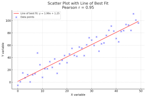
To represent the Pearson correlation coefficient with a plot, we typically create a scatter plot of the two variables and add the line of best fit to visualize the linear relationship. The slope of the line and how closely the points cluster around the line give a visual indication of the strength and direction of the linear relationship. The following is the plot:
Here’s the scatter plot with a line of best fit for a dataset with a positive linear relationship. The Pearson correlation coefficient (r) is annotated on the plot, indicating the strength and direction of the linear relationship between the x and y variables.
The line of best fit gives a visual representation of this relationship, and the scatter of points around the line indicates how closely they follow a linear pattern. The closer the Pearson coefficient is to 1, the stronger the positive linear relationship between the variables.
The Spearman correlation coefficient is used to represent relationship between the variables in the non-normal monotonic dataset. The following plots represent the non-normal monotonic dataset with or without outliers.
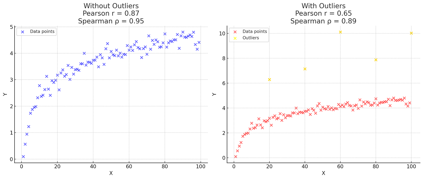
In the visualizations:
- Left Plot (Without Outliers): This plot shows the dataset without outliers, and both Pearson and Spearman correlation coefficients are relatively high, indicating a strong monotonic relationship. Since the data is non-normal and monotonic, both coefficients show similar strength due to the lack of outliers and the overall pattern of the data.
- Right Plot (With Outliers): Here, the data consists of few outliers. You can see that the Pearson correlation coefficient has dropped significantly due to the presence of these outliers. This is because Pearson’s correlation is heavily influenced by the actual values, and outliers can have a large impact on the result. In contrast, the Spearman correlation coefficient has not been affected as much by the outliers because it relies on the rank order of the data, which is less sensitive to extreme values.
Whether to Choose Pearson or Spearman Correlation Coefficient?
Selecting the appropriate method (Spearman vs Pearson) to measure correlation requires careful consideration of various aspects of the data.
Determining the Scale of Measurement in Your Data Firstly, it’s essential to identify the scale of measurement. Pearson’s correlation is suitable for data measured on an interval or ratio scale—where the intervals between data points are equal. Examples include temperature in Celsius or revenue in dollars. Spearman’s correlation is apt for ordinal data or interval/ratio data that do not meet the normality assumption. An example of ordinal data could be a rating scale from 1 to 5, as discussed previously.
Assessing the Relationship Between Variables The nature of the relationship between variables is another critical factor. If the relationship is linear, meaning that the change in one variable is proportionally associated with a change in another, Pearson’s correlation should be used. If the relationship is monotonic, where the variables tend to move in the same direction but not necessarily at a constant rate, Spearman’s correlation is more appropriate.
Dealing with Outliers and Non-normal Distributions Outliers can significantly impact the results of a Pearson correlation analysis. If your data contains outliers or is not normally distributed, Spearman’s correlation, which uses ranks rather than actual values, can provide a more accurate measure of the relationship.
There is no one-size-fits-all approach when choosing between Pearson and Spearman correlation coefficients. Each dataset should be evaluated on its own merits, and the choice should be justified based on the characteristics of the data and the specific research questions posed.

Check out my latest book titled as First Principles Thinking: Building winning products using first principles thinking.
- Mathematics Topics for Machine Learning Beginners - July 6, 2025
- Questions to Ask When Thinking Like a Product Leader - July 3, 2025
- Three Approaches to Creating AI Agents: Code Examples - June 27, 2025
I found it very helpful. However the differences are not too understandable for me