
Generalized linear models (GLMs) are a powerful tool for data scientists, providing a flexible way to model data. In this post, you will learn about the concepts of generalized linear models (GLM) with the help of Python examples. It is very important for data scientists to understand the concepts of generalized linear models and how are they different from general linear models such as regression or ANOVA models.
What are Generalized Linear Models?
Generalized linear models (GLM) are a type of statistical models that can be used to model data that is not normally distributed. It is a flexible general framework that can be used to build many types of regression models, including linear regression, logistic regression, and Poisson regression. GLM provides a way to model dependent variables that have non-normal distributions. GLM also allows for the incorporation of predictor variables that are not Normally distributed. GLMs are similar to linear regression models, but they can be used with data that has a non-normal distribution. This makes GLMs a more versatile tool than linear regression models. This is different from the general linear models (linear regression / ANOVA) where response variable, Y, and the random error term ([latex]\epsilon[/latex]) have to be based solely on the normal distribution. Linear models can be expressed in terms of expected value (mean) of response variable as the following:
[latex]\Large g(\mu)= \sum\limits_{i=1}^n \beta_iX_i[/latex] … where [latex]\mu[/latex] can be expressed as E(Y) aka expected value of response variable Y.
.
Based on the probability distribution of the response variable, different link functions get used which transforms [latex]g(\mu)[/latex] appropriately to the output value which gets modeled using different types of regression models. If the response variable is normally distributed, the link function is identify function and the model looks like the following. Y, in the equation below, represents the expected value or E(Y).
[latex]\Large Y = \sum\limits_{i=1}^n \beta_iX_i[/latex]
GLM can be used for both regression and classification problems. In regression, the goal is to predict the value of the dependent variable (e.g., price of a house). In classification, the goal is to predict the class label of the dependent variable (e.g., whether a patient has cancer).
Before getting into generalized linear models, lets quickly understand the concepts of general linear models.
What are General Linear Models?
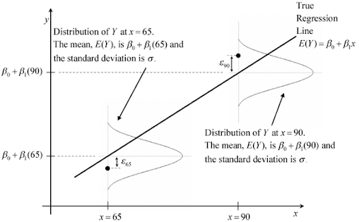
General linear models are the models which is used to predict the value of continuous response variable and, at any given predictor value, X, the response variable, Y, and random error term ([latex]\epsilon[/latex]) follows a normal distribution. The parameter of such normal distribution represents the mean as linear combination of weights (W) and predictor variable (X), and, the standard deviation of [latex]\sigma[/latex]. Linear regression and ANOVA models represent the general linear models. The diagram given below represents the same in form of simple linear regression model where there is just one coefficient.
For linear regression models, the link function is identity function. Recall that a link function transforms the probabilities of the levels of a categorical response variable to a continuous scale that is unbounded. Once the transformation is complete, the relationship between the predictors and the response can be modeled with linear regression. Thus, the linear combination of weights and predictor variable is modelled as output. The linear regression models using identity function as link function can be understood as the following:
[latex]\Large Y_{actual} = Y_{predicted} + \epsilon[/latex] … The actual value is the sum of predicted value and the random error term (which can be on either side of the mean value – response value)
.
[latex]\Large Y_{actual} = \sum\limits_{i=1}^n \beta_iX_i + \epsilon[/latex]
.
As part of training regression models, one must understand that what is actually modelled is the mean of the response variable values and not the actual values. As the response variable Y follows normal distribution, the summation of weights and predictor variable can be equated as the expected value of Y.
[latex]\Large E(Y) = \sum\limits_{i=1}^n \beta_iX_i[/latex]
.
The actual value of Y can be represented as the following in terms of outcome from regression model and the random error term:
[latex]\Large Y_{actual} = E(Y) + \epsilon[/latex]
.
For the linear regression model, the identity function is link function used to link the mean of expected value of response variable, Y, and the summation of weights and predictor variable. Thus, the g(E(Y)) becomes E(Y) which is represented as [latex]Y_{predicted}[/latex]. Thus, linear regression model (also, at times termed as general linear models) is represented as the following:
[latex]\Large Y_{predicted} = \sum\limits_{i=1}^n \beta_iX_i[/latex]
Given above, lets understand what are generalized linear models.
What are Generalized Linear Models (GLM)?
In generalized linear models, the link function used to model the response variable as a function of the predictor variables are the following. Note that the Y represents the mean or expected value of the response variable.
- Log Link: Log(Y) – Models the logarithm of mean Y. Thus, the regression model can be represented as the following:
[latex]\Large Log(Y) = \sum\limits_{i=1}^n \beta_iX_i[/latex] … This type of regression model is called as Poisson regression. It is used to model the non-negative count value as in Poisson probability distribution.
.
- Logit Link: [latex]Log(\frac{Y}{(1 – Y)})[/latex] – Models the logarithm of odds of the probability of binary outcome. Thus, the regression model can be represented as the following:
[latex]\Large Log(\frac{Y}{(1 – Y)})= \sum\limits_{i=1}^n \beta_iX_i[/latex] .. This type of regression model is called as Logistic regression. It is used to model the probability of the binary outcome.
.
- There are other link functions which result in modeling response variable based on gamma distribution (GammaRegressor), Tweedie distribution (TweedieRegressor) etc.
The above regression models used for modeling response variable with Poisson, Gamma, Tweedie distribution etc are called as Generalized Linear Models (GLM).
Generalized Linear Models Examples
Here are some real-world examples where generalized linear models can be used to predict continuous response variables based on their probability distribution. The table consists of reference to the SKlearn class which can be used to model the response variables.
| Problem Type | Example | Regression Model (Sklearn) |
| Agriculture / weather modeling | Number of rain events per year | PoissonRegressor |
| Agriculture / weather modeling | Amount of rainfall per rainfall event | GammaRegressor |
| Agriculture / weather modeling | Total rainfall per year | TweedieRegressor |
| Risk modeling / insurance policy pricing | No of claim events / policyholder per year | PoissonRegressor |
| Risk modeling / insurance policy pricing | Cost per claim event | GammaRegressor |
| Risk modeling / insurance policy pricing | Total cost per policyholder | TweedieRegressor |
| Predictive maintenance | Number of production interruption events per year | PoissonRegressor |
| Predictive maintenance | Duration of interruption | GammaRegressor |
| Predictive maintenance | Total interruption time per year | TweedieRegressor |
When to use Generalized Linear Models (GLM)?
Generalized linear models of different kinds are used based on the probability distribution of the response variables.
- GLM is particularly useful when the response variable is not normally distributed or when the relationship between the predictor variables and the response variable is non-linear.
- If the response variable represents counts (non-negative integer valued) or relative frequencies (non-negative), Poisson regression with log-link is used. Sklearn PoissonRegressor can be used to model such response variable.
- If the response variable values are positive valued and skewed, Sklearn GammaRegressor with log-link can be tried.
- If the response variable values seem to be heavier tailed than a Gamma distribution, one may try an Inverse Gaussian distribution based regressor such as Sklearn TweedieRegressor.
- If the response variable is related to binary outcome, Logistic regression with Logit link can be used. Sklearn LogisticRegression can be used to model the response variable having binary outcome.
- GLM allows for the inclusion of interaction terms and polynomial terms. As a result, GLM is a versatile tool that can be used in a wide range of situations.
Conclusions
Here is the summary of what you learned in this post in relation to generalized linear models:
- Generalized linear models are used to model the response variable as a linear combination of weights and predictor variable given the response variable and the error term follows the exponential family of distributions.
- GLM can model response variable which follows distribution such as normal, Poisson, Gamma, Tweedie, binomial etc.
- Python Sklearn provides classes to train GLM models depending upon the probability distribution followed by the response variable.

Check out my latest book titled as First Principles Thinking: Building winning products using first principles thinking.
- Mathematics Topics for Machine Learning Beginners - July 6, 2025
- Questions to Ask When Thinking Like a Product Leader - July 3, 2025
- Three Approaches to Creating AI Agents: Code Examples - June 27, 2025
I found it very helpful. However the differences are not too understandable for me