
Linear regression is a simple and widely used statistical method for modeling relationships between variables. While it can be applied to time-series data for trend analysis and basic forecasting, it is not always the most apt method for time-series forecasting due to several limitations.
Forecasting using Linear Regression
Forecasting using linear regression involves using historical data to predict future values based on the assumption of a linear relationship between the independent variable (time) and the dependent variable (the metric to be forecasted, like CO2 levels discussed in next section). The process typically involves the following steps:
- Data Preparation: Organize the data in a time series format, where one variable represents time, and the other represents the variable to forecast. The following aspects need to be addressed at this stage:
- Stationarity: Ensure the data is stationary. This means the mean, variance, and autocorrelation should remain constant over time. Techniques like differencing and detrending can be used to achieve stationarity.
- Feature Engineering: Create additional features based on the existing data, such as lagged values or time-based features like day of the week or month.
- Model Fitting: Apply linear regression to fit a line through the data points. The model estimates coefficients for the intercept and the slope, which defines the best-fit line.
- Prediction: Use the regression model to predict future values by extending the time variable beyond the range of the historical data and applying the regression formula.
- Evaluation: Assess the model’s accuracy using metrics like R-squared, Mean Squared Error (MSE), or others.
Limitations for Linear Regression used in Forecasting
- Assumes linearity: It only captures linear relationships between variables. Real-world time-series datasets, especially those in fields like finance, economics, and environmental science, often exhibits non-linear patterns, limiting its accuracy.
- Ignoring Autocorrelation: Time-series data often exhibit autocorrelation, meaning that a value at a given time is correlated with its past values. Linear regression does not account for this autocorrelation, which can lead to inaccurate forecasts, particularly for longer forecast horizons.
- Limited to short-term forecasts: As time progresses, non-linear factors become more influential, reducing its effectiveness for long-term forecasting.
- Requires stationary data: Non-stationary data needs pre-processing, which can be complex and affect accuracy.
- Seasonality and Trend: Time-series data often contain trends and seasonal patterns. Linear regression does not inherently account for these unless explicitly modeled, which can complicate the model and reduce its effectiveness.
- Vulnerability to Outliers: Linear regression can be sensitive to outliers, which are common in time-series data. Outliers can significantly affect the slope and intercept of the regression line, leading to inaccurate predictions.
Is linear regression most efficient method for Forecasting?
While linear regression is straightforward and easy to understand, it is not always the most efficient method for forecasting, especially for complex time series. Its major limitations are listed in the previous section. The following are some other model choices that may work better:
- Exponential Smoothing: Suitable for short-term forecasts and capturing trends/seasonality.
- ARIMA (Autoregressive Integrated Moving Average): Powerful for stationary data with strong autocorrelation.
- Deep learning models such as LSTMs (Long Short-Term Memory): Handles non-linear patterns and long-term dependencies in complex data.
- Prophet: Facebook’s open-source forecasting tool, suitable for multiple time series formats.
Deciding Linear Regression Suitability for Forecasting
Deciding whether linear regression is an apt method for forecasting in a given situation involves assessing several key aspects of your data and the nature of your forecasting requirement. Here are the three most important rules:
- Short-Term Forecasting: While linear regression can handle short-term forecasts well, its accuracy diminishes for long-term predictions. As time progresses, non-linear factors become more influential, making linear models less reliable for long-term forecasting. Consider other methods like ARIMA or LSTMs for longer timeframes.
- Linear Relationship: The most crucial rule is that linear regression can only capture linear relationships. Analyze your data for linearity. If you observe a linear trend or a strong correlation between your independent and dependent variables, linear regression might be suitable. However, if the relationship appears non-linear (e.g., exponential, cyclical), linear regression will not give accurate forecasts. Plot the data to visualize the relationship. Linear regression forecast accuracy relies on this assumption.
- Stationarity: Linear regression requires stationary data, meaning the mean, variance, and autocorrelation remain constant over time. Non-stationary data needs pre-processing like differencing or detrending. If your data exhibits trends, seasonality, or other non-stationary patterns, linear regression might not be the best choice.
Additionally, here are some other useful checks before settling on a linear forecasting model:
- Residual Analysis: After fitting a linear model, analyze the residuals – the differences between the observed values and the model’s predictions. Ideally, residuals should be randomly distributed with no discernible pattern. Non-random patterns in residuals can indicate that the linear model is not capturing all the underlying relationships in the data. Check for homoscedasticity, meaning the variance of residuals is constant across all values of the independent variable. If not homoscedastic, consider transformations or weighted least squares. After fitting the model, plot the residuals against the independent variable and time. Analyze for any patterns or trends.
- Model Comparison: Compare the performance of the linear regression model with other forecasting methods like exponential smoothing, ARIMA, or LSTMs. Use metrics like mean squared error (MSE), root mean squared error (RMSE), and mean absolute error (MAE) to compare the performance of different models.
Python Example Implementation for Forecasting using Linear Regression
We will look into the Python implementation for forecasting using linear regression while working with Sklearn dataset, Mauna Loa CO2 data.
The Mauna Loa CO2 dataset, recording atmospheric carbon dioxide concentrations, is pivotal for understanding the escalating CO2 levels in our atmosphere, a key indicator of climate change. This dataset not only reveals a worrying upward trend signaling ongoing and possibly accelerating climate change but also exhibits seasonal fluctuations due to natural cycles like plant growth and decay. These variances are crucial for accurate data interpretation, necessitating sophisticated representation methods to capture the complex interplay of natural and human-driven factors.
Forecasting future CO2 trends using this data is essential for various reasons. It aids in climate modeling and making informed predictions about future climate impacts, guiding scientists and policymakers. Accurate forecasts are critical in shaping policies and international agreements aimed at CO2 emission reduction, setting realistic targets, and measuring the effectiveness of carbon reduction strategies. Understanding and predicting long-term CO2 trends is vital for preparing for their far-reaching effects on weather patterns, sea levels, ecosystems, and agriculture.
from sklearn.datasets import fetch_openml
from sklearn.linear_model import LinearRegression
import matplotlib.pyplot as plt
import pandas as pd
import numpy as np
from datetime import datetime, timedelta

# Fetching the Mauna Loa CO2 data
data = fetch_openml('mauna-loa-atmospheric-co2', as_frame=True)

# Creating a timestamp column
data['data']['timestamp'] = data['data'].apply(lambda row: datetime(int(row['year']), int(row['month']), int(row['day'])), axis=1)

# Converting timestamp to ordinal to use in linear regression
data['data']['ordinal'] = data['data']['timestamp'].apply(lambda x: x.toordinal())

# Splitting the dataset into features and target variable
X = data['data']['ordinal'].to_numpy().reshape(-1, 1)
y = data['target'].to_numpy()

# Creating and fitting a linear regression model
model = LinearRegression()
model.fit(X, y)

# Preparing data for forecasting
last_date = data['data']['timestamp'].iloc[-1]
forecast_years = 5
future_dates = [last_date + timedelta(days=i) for i in range(1, forecast_years * 365)]
future_ordinals = np.array([d.toordinal() for d in future_dates]).reshape(-1, 1)

# Predicting CO2 levels for future dates
future_pred = model.predict(future_ordinals)

# Plotting CO2 levels and the regression line over time, including forecast
plt.figure(figsize=(12, 6))
plt.plot(data['data']['timestamp'], y, label='CO2 Levels')
plt.plot(data['data']['timestamp'], model.predict(X), color='red', label='Regression Line')
plt.plot(future_dates, future_pred, color='green', linestyle='dashed', label='Forecast')
plt.xlabel('Year')
plt.ylabel('CO2 levels (ppm)')
plt.title('CO2 Levels Over Time with Linear Regression Line and Forecast at Mauna Loa Observatory')
plt.legend()
plt.show()
Here is the plot that gets created:
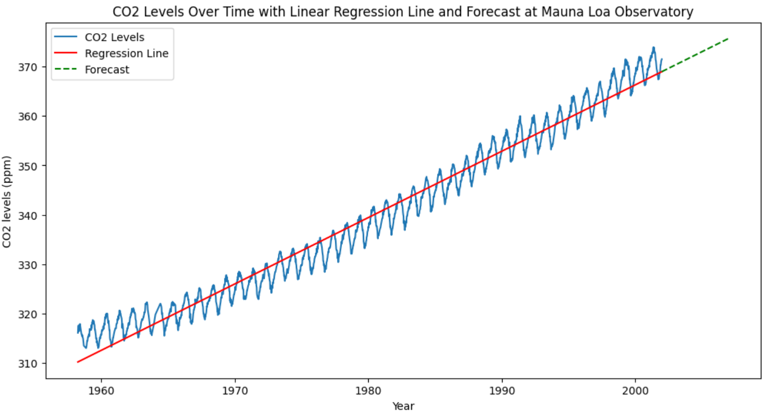
In the above Python code, the predictions are plotted as a green dashed line to distinguish them from the actual data and the regression line. This approach provides a simple linear extrapolation of the current trend into the future. However, it’s important to note that linear regression is quite basic and might not accurately capture more complex patterns in the data, such as nonlinear trends or seasonal variations. For more accurate forecasting, more sophisticated time-series models would be required.

Check out my latest book titled as First Principles Thinking: Building winning products using first principles thinking.
- Three Approaches to Creating AI Agents: Code Examples - June 27, 2025
- What is Embodied AI? Explained with Examples - May 11, 2025
- Retrieval Augmented Generation (RAG) & LLM: Examples - February 15, 2025
I found it very helpful. However the differences are not too understandable for me