A feedforward neural network, also known as a multi-layer perceptron, is composed of layers of neurons that propagate information forward. In this post, you will learn about the concepts of feedforward neural network along with Python code example. We will start by discussing what a feedforward neural network is and why they are used. We will then walk through how to code a feedforward neural network in Python. In order to get good understanding on deep learning concepts, it is of utmost importance to learn the concepts behind feed forward neural network in a clear manner. Feed forward neural network learns the weights based on backpropagation algorithm which will be discussed in future posts.
What’s Feedforward Neural Network?
Feed forward neural network represents the mechanism in which the input signals fed forward into a neural network, passes through different layers of the network in form of activations and finally results in form of some sort of predictions in the output layer. Here is an animation representing the feed forward neural network which classifies input signals into one of the three classes shown in the output.
Note some of the following aspects in the above animation in relation to how the input signals (variables) are fed forward through different layers of the neural network:
- The neural network shown in the animation consists of 4 different layers – one input layer (layer 1), two hidden layers (layer 2 and 3) and one output layer (layer 4).
- Input fed into input layer: There are four input variables which are fed into different nodes in the the neural network through input layer (1st layer). No computations happen in the input layer.
- Activations in first hidden layer: Sum of Input signals (variables) combined with weights and a bias element are fed into all the neurons of first hidden layer (layer 2). At each neuron, all incoming values are added together (weighted sum of input signals) and then fed into an activation function (such as relu, tanh, sigmoid function etc). Read about different activation functions in this post – Activation functions in neural network. Based on whether the output of activation function is more than a threshold value decides whether the neuron gets activated / fired or not. In the first hidden layer, note that only four neurons get activated / fired. The hidden layer can be seen to learn the data representation to be fed into next hidden layer. These data representation tends to learn the interaction between the features.
- Activations in second hidden layer: The activation signals from layer 2 (first hidden layer) are then combined with weights, added with a bias element, and fed into layer 3 (second hidden layer). At each neuron in layer three, all incoming values (weighted sum of activation signals) are added together and then processed with an activation function same as that used in layer 2. This is why this neural network can be termed fully connected neural network. Based on whether the output of activation function is more than a threshold value decides whether the neuron gets activated / fired or not. In the second hidden layer, note that only three neurons get activated / fired.
- Softmax output in the final layer: Finally, the activation signals from second hidden layer are combined with weights and fed into the output layer. At each node in the final / output layer, all incoming values (weighted sum of activation signals) are added together in different nodes and then processed with a function such as softmax function to output the probabilities (in case of classification).
In feedforward neural network, the value that reaches to the new neuron is the sum of all input signals and related weights if it is first hidden layer, or, sum of activations and related weights in the neurons in the next layers.
For top-most neuron in the first hidden layer in the above animation, this will be the value which will be fed into the activation function. You may want to check out my other post on how to represent neural network as mathematical model.
[latex]weightedSum = \theta^{(1)}_{10}x_0 + \theta^{(1)}_{11}x_1 + \theta^{(1)}_{12}x_2 + \theta^{(1)}_{13}x_3 + \theta^{(1)}_{14}x_4[/latex]
.
For the top-most neuron in the second layer in the above animation, this will be the value of weighted sum which will be fed into the activation function:
[latex]weightedSum = \theta^{(2)}_{10}a^{(1)}_0 + \theta^{(2)}_{11}a^{(1)}_1 + \theta^{(2)}_{12}a^{(1)}_2 + \theta^{(2)}_{13}a^{(1)}_3 + \theta^{(2)}_{14}a^{(1)}_4 + \theta^{(2)}_{15}a^{(1)}_5 + \theta^{(2)}_{16}a^{(1)}_6[/latex]
.
Finally, this will be the output reaching to the first / top-most node in the output layer.
[latex]weightedSum = \theta^{(3)}_{10}a^{(2)}_0 + \theta^{(3)}_{11}a^{(2)}_1 + \theta^{(3)}_{12}a^{(2)}_2 + \theta^{(3)}_{13}a^{(2)}_3 + \theta^{(3)}_{14}a^{(2)}_4 + \theta^{(3)}_{15}a^{(2)}_5 + \theta^{(3)}_{16}a^{(2)}_6[/latex]
.
Based on the above formula, one could determine weighted sum reaching to every node / neuron in every layer which will then be fed into activation function.
The picture below (computational graph) represents how the value of objective function is calculated for a feedforward multi-layer perceptron neural network with one hidden layer. The diagram is taken from this page on dive into deep learning website.
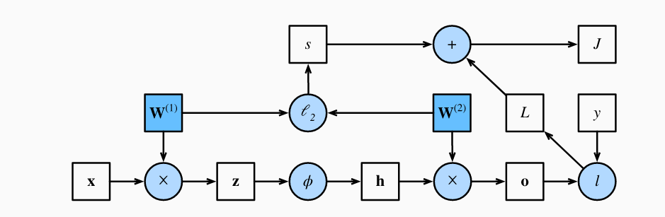
Note some of the following in the above picture:
- Weighted sum represented as z is fed into activation function
- Activation function output h is combined with another weights and weighted sum is fed into output function o
- Loss l is calculated by comparing output value (function o) with actual value (y)
- The loss is then combined with the L2 normalization (represented using s) and then the objective function is calculated
Feedforward Neural Network Python Example
In this section, you will learn about how to represent the feed forward neural network using Python code.
As a first step, let’s create sample weights to be applied in the input layer, first hidden layer and the second hidden layer. Here is the code. Note that the weights for each layer is created as matrix of size M x N where M represents the number of neurons in the layer and N represents number of nodes / neurons in the next layer. Thus, the weight matrix applied to the input layer will be of size 4 X 6. Weights matrix applied to activations generated from first hidden layer is 6 X 6. Weights matrix applied to activations generated from second hidden layer is 6 X 4.
import numpy as np
from sklearn import datasets
#
# Generate a dataset and plot it
#
np.random.seed(0)
X, y = datasets.make_moons(200, noise=0.20)
#
# Neural network architecture
# No of nodes in input layer = 4
# No of nodes in output layer = 3
# No of nodes in the hidden layer = 6
#
input_dim = 4 # input layer dimensionality
output_dim = 3 # output layer dimensionality
hidden_dim = 6 # hidden layer dimensionality
#
# Weights and bias element for layer 1
# These weights are applied for calculating
# weighted sum arriving at neurons in 1st hidden layer
#
W1 = np.random.randn(input_dim, hidden_dim)
b1 = np.zeros((1, hidden_dim))
#
# Weights and bias element for layer 2
# These weights are applied for calculating
# weighted sum arriving at neurons in 2nd hidden layer
#
W2 = np.random.randn(hidden_dim, hidden_dim)
b2 = np.zeros((1, hidden_dim))
#
# Weights and bias element for layer 2
# These weights are applied for calculating
# weighted sum arriving at in the final / output layer
#
W3 = np.random.randn(hidden_dim, output_dim)
b3 = np.zeros((1, output_dim))
Let’s see the Python code for propagating input signal (variables value) through different layer to the output layer. Pay attention to some of the following:
- Weighted sum is calculated for neurons at every layer. Note that weighted sum is sum of weights and input signal combined with the bias element.
- Softmax function is applied to the output in the last layer.
#
# Forward propagation of input signals
# to 6 neurons in first hidden layer
# activation is calculated based tanh function
#
z1 = X.dot(W1) + b1
a1 = np.tanh(z1)
#
# Forward propagation of activation signals from first hidden layer
# to 6 neurons in second hidden layer
# activation is calculated based tanh function
#
z2 = a1.dot(W2) + b2
a2 = np.tanh(z2)
#
# Forward propagation of activation signals from second hidden layer
# to 3 neurons in output layer
#
z3 = a2.dot(W3) + b3
#
# Probability is calculated as an output
# of softmax function
#
probs = np.exp(z3) / np.sum(np.exp(z3), axis=1, keepdims=True)
Conclusions
Here is the summary of what you learned in this post in relation for feed forward neural network:
- Feed forward neural network represents the aspect of how input to the neural network propagates in different layers of neural network in form of activations, thereby, finally landing in the output layer.
- All the layers except the last one (output layer) can be understood as the layers which are used to learn the data representations (features), especially, interaction between the features.
- Input signals arriving at any particular neuron / node in the inner layer is sum of weighted input signals combined with bias element. The particular node transmits the signal further or not depends upon whether the combined sum of weighted input signal and bias is greater than a threshold value or not.

Check out my latest book titled as First Principles Thinking: Building winning products using first principles thinking.
- Three Approaches to Creating AI Agents: Code Examples - June 27, 2025
- What is Embodied AI? Explained with Examples - May 11, 2025
- Retrieval Augmented Generation (RAG) & LLM: Examples - February 15, 2025
Dear Mr Ajitesh Kumar :
I run the code that you gave. When in >>> z1 = X.dot(W1) + b1 I pressed Enter Key showing the error message like “ValueError: shapes (200,2) and (4,6) not aligned: 2 (dim 1) != 4 (dim 0) ”
What is wrong ? why not (200,4) to match with (4,6) I do not know number 2 in shape(200,2) what it come from. Could you please help me to solve the problem. Thank you, Kuntoro Kuntoro Division of Biostatistics and Population Study Airlangga University School of Public Health Surabaya Indonesia