
Last updated: 17 Sept, 2024
Principal component analysis (PCA)is a dimensionality reduction technique that reduces the number of dimensions or features in a dataset without sacrificing a lot of information. What if it is told that you could take a dataset with 500 columns, use PCA to reduce it to 50 columns, and still able to retain 90% or more of the information in the original dataset? Wouldn’t that sound like a miracle?
In this post, you will learn about how to use PCA for extracting important features (also termed as feature extraction technique) from a list of given features. As a machine learning / data scientist, it is very important to learn the PCA technique for feature extraction as it helps you visualize the data in the lights of importance of explained variance of data set. The following topics get covered in this post:
- What is principal component analysis?
- PCA algorithm for feature extraction
- PCA Python implementation step-by-step
- PCA Python Sklearn example
What is Principal Component Analysis?
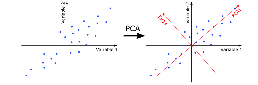
Principal component analysis (PCA) is an unsupervised linear transformation technique which is primarily used for dimensionality reduction and feature extraction. It aims to find the directions of maximum variance in high-dimensional data and projects the data onto a new subspace with equal or fewer dimensions than the original one. In the diagram given below, note the directions of maximum variance of data. This is represented using PCA1 (first maximum variance) and PC2 (2nd maximum variance).
It is the direction of maximum variance of data that helps us identify an object. For example, in a movie, it is okay to identify objects by 2-dimensions as these dimensions represent direction of maximum variance. Take a look at a real-world example of understanding direction of maximum variance in the following picture representing Taj Mahal of Agra. The diagram below represents the side view of Taj Mahal. There are multiple dimensions consisting of information (maximum variance) which helps identify the picture as Taj Mahal.

Fig 2. Taj Mahal Side View
Take a look the following picture of Taj Mahal from top view. Note that there are only fewer dimensions in which information is varying and the variance is also not much. Hence, it is difficult to identify from top view whether the picture is of Taj Mahal. Thus, top view can be ignored easily.

Fig 3. Taj Mahal Top View
Thus, when training a model to classify whether a given structure is of Taj Mahal or not, one would want to ignore the dimensions / features related to top view as they don’t provide much information (as a result of low variance).
How is PCA different than other feature selection techniques?
The way PCA is different from other feature selection techniques such as random forest, regularization techniques, forward/backward selection techniques etc is that it does not require class labels to be present (thus called as unsupervised). More details along with Python code example will be shared in future posts.
PCA Algorithm for Feature Extraction
The following represents 6 steps of principal component analysis (PCA) algorithm:
- Standardize the dataset: Standardizing / normalizing the dataset is the first step one would need to take before performing PCA. The PCA calculates a new projection of the given data set representing one or more features. The new axes are based on the standard deviation of the value of these features. So, a feature / variable with a high standard deviation will have a higher weight for the calculation of axis than a variable / feature with a low standard deviation. If the data is normalized / standardized, the standard deviation of all fetaures / variables get measured on the same scale. Thus, all variables have the same weight and PCA calculates relevant axis appropriately. Note that the data is standardized / normalized after creating training / test split. Python’s sklearn.preprocessing StandardScaler class can be used for standardizing the dataset.
- Construct the covariance matrix: Once the data is standardized, the next step is to create n X n-dimensional covariance matrix, where n is the number of dimensions in the dataset. The covariance matrix stores the pairwise covariances between the different features. Note that a positive covariance between two features indicates that the features increase or decrease together, whereas a negative covariance indicates that the features vary in opposite directions. Python‘s Numpy cov method can be used to create covariance matrix.
- Perform Eigendecomposition of covariance matrix: The next step is to decompose the covariance matrix into its eigenvectors and eigenvalues. The eigenvectors of the covariance matrix represent the principal components (the directions of maximum variance), whereas the corresponding eigenvalues will define their magnitude. Numpy linalg.eig or linalg.eigh can be used for decomposing covariance matrix into eigenvectors and eigenvalues.
- Selection of most important Eigenvectors / Eigenvalues: Sort the eigenvalues by decreasing order to rank the corresponding eigenvectors. Select k eigenvectors, which correspond to the k largest eigenvalues, where k is the dimensionality of the new feature subspace (
). One can used the concepts of explained variance to select the k most important eigenvectors.
- Projection matrix creation of important eigenvectors: Construct a projection matrix, W, from the top k eigenvectors.
- Training / test dataset transformation: Finally, transform the d-dimensional input training and test dataset using the projection matrix to obtain the new k-dimensional feature subspace.
PCA Python Implementation Step-by-Step
This section represents custom Python code for extracting the features using PCA. The Kaggle campus recruitment dataset is used.
Here are the steps followed for performing PCA:
- Perform one-hot encoding to transform categorical data set to numerical data set
- Perform training / test split of the dataset
- Standardize the training and test data set
- Construct covariance matrix of the training data set
- Construct eigendecomposition of the covariance matrix
- Select the most important features using explained variance
- Construct project matrix; In the code below, the projection matrix is created using the five eigenvectors that correspond to the top five eigenvalues (largest), to capture about 75% of the variance in this dataset
- Transform the training data set into new feature subspace
Here is the custom Python code (without using sklearn.decomposition PCA class) to achieve the above PCA algorithm steps for feature extraction:
#
# Perform one-hot encoding
#
categorical_columns = df.columns[df.dtypes == object] # Find all categorical columns

df = pd.get_dummies(df, columns = categorical_columns, drop_first=True)
#
# Create training / test split
#
from sklearn.model_selection import train_test_split
X_train, X_test, y_train, y_test = X_train, X_test, y_train, y_test = train_test_split(df[df.columns[df.columns != 'salary']],
                   df['salary'], test_size=0.25, random_state=1)
#
# Standardize the dataset; This is very important before you apply PCA
#
from sklearn.preprocessing import StandardScaler
sc = StandardScaler()
sc.fit(X_train)
X_train_std = sc.transform(X_train)
X_test_std = sc.transform(X_test)
#
# Import eigh method for calculating eigenvalues and eigenvectirs
#
from numpy.linalg import eigh
#
# Determine covariance matrix
#
cov_matrix = np.cov(X_train_std, rowvar=False)
#
# Determine eigenvalues and eigenvectors
#
egnvalues, egnvectors = eigh(cov_matrix)
#
# Determine explained variance and select the most important eigenvectors based on explained variance
#
total_egnvalues = sum(egnvalues)
var_exp = [(i/total_egnvalues) for i in sorted(egnvalues, reverse=True)]
#
# Construct projection matrix using the five eigenvectors that correspond to the top five eigenvalues (largest), to capture about 75% of the variance in this dataset
#
egnpairs = [(np.abs(egnvalues[i]), egnvectors[:, i])
                for i in range(len(egnvalues))]
egnpairs.sort(key=lambda k: k[0], reverse=True)
projectionMatrix = np.hstack((egnpairs[0][1][:, np.newaxis],
                              egnpairs[1][1][:, np.newaxis],
                              egnpairs[2][1][:, np.newaxis],
                              egnpairs[3][1][:, np.newaxis],
                              egnpairs[4][1][:, np.newaxis]))
#
# Transform the training data set
#
X_train_pca = X_train_std.dot(projectionMatrix)
PCA Python Sklearn Example
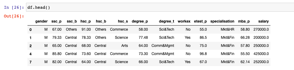
This section represents Python code for extracting the features using sklearn.decomposition class PCA. The Kaggle campus recruitment dataset is used. Here is the screenshot of the data used. Salary is the label. The goal is to predict the salary.
Here are the steps followed for performing PCA:
- Perform one-hot encoding to transform categorical data set to numerical data set
- Perform training / test split of the dataset
- Standardize the training and test data set
- Perform PCA by fitting and transforming the training data set to the new feature subspace and later transforming test data set.
- As a final step, the transformed dataset can be used for training/testing the model
Here is the Python code to achieve the above PCA algorithm steps for feature extraction:
#
# Perform one-hot encoding
#
categorical_columns = df.columns[df.dtypes == object] # Find all categorical columns

df = pd.get_dummies(df, columns = categorical_columns, drop_first=True)
#
# Create training / test split
#
from sklearn.model_selection import train_test_split
X_train, X_test, y_train, y_test = X_train, X_test, y_train, y_test = train_test_split(df[df.columns[df.columns != 'salary']],
                   df['salary'], test_size=0.25, random_state=1)
#
# Standardize the dataset; This is very important before you apply PCA
#
from sklearn.preprocessing import StandardScaler
sc = StandardScaler()
sc.fit(X_train)
X_train_std = sc.transform(X_train)
X_test_std = sc.transform(X_test)
#
# Perform PCA
#
from sklearn.decomposition import PCA
pca = PCA()
#
# Determine transformed features
#
X_train_pca = pca.fit_transform(X_train_std)
X_test_pca = pca.transform(X_test_std)
Benefits of using PCA Technique in Machine Learning
The following are some of the benefits of using PCA techniques:
- Data Exploration using Potting: PCA is often used for reducing high-dimensional data to two or three dimensions, plot the data and learn about the relationship.
- Data Anonymization: PCA can as well be used to anonymize the datasets so that they can be shared with others without revealing the nature or meaning of the data
- PCa can be used for reducing the number of dimensions in a dataset and then restoring the original number of dimensions. This finds application in anomaly detection and noise filtering.
- PCA helps in Anomaly Detection: PCA-based reconstruction is especially useful in anomaly detection. The idea is that, in normal data, the approximation error (difference between the original and reconstructed data) is small because PCA captures the most important variance. However, anomalies, which do not follow the usual data patterns, will have a larger reconstruction error. By monitoring this error, anomalies can be detected.
- PCA helps in noise filtering: In noise filtering, PCA can be used to remove noise from the data by discarding the dimensions that correspond to less significant principal components (which typically capture noise). The reconstruction from the top components will yield a version of the data with reduced noise, as only the significant variance (i.e., the main patterns) is retained.
Conclusions
Here is the summary of what you learned in relation to applying principal component analysis (PCA) for feature extraction.
- Feature extraction is about transforming features into new feature subspace while retaining information in original features.
- New features subspace is created by transforming d-dimensional data set into k-dimensional data set by using projection matrix. Projection matrix is constructed by selecting K most important eigenvectors.
- Most important eigenvectors are selected by sorting eigenvalues and finding their explained variance ratio.
- Eigenvectors & eigenvalues are created by doing eigendecomposition of covariance matrix of original data set.
- Before performing PCA, the data set must be standardized.
- There are several benefits of using PCA including data exploration, data anonymization, solving problems related to anomaly detection & noise filtering, etc.

Check out my latest book titled as First Principles Thinking: Building winning products using first principles thinking.
- Mathematics Topics for Machine Learning Beginners - July 6, 2025
- Questions to Ask When Thinking Like a Product Leader - July 3, 2025
- Three Approaches to Creating AI Agents: Code Examples - June 27, 2025
I found it very helpful. However the differences are not too understandable for me