In this post, you will understand the key differences between Adaline (Adaptive Linear Neuron) and Logistic Regression.
- Activation function
- Cost function
Difference in Activation Function
The primary difference is the activation function. In Adaline, the activation function is called as linear activation function while in logistic regression, the activation function is called as sigmoid activation function. The diagram below represents the activation functions for Adaline. The activation function for Adaline, also called as linear activation function, is the identity function which can be represented as the following:
$$\phi(W^TX) = W^TX$$
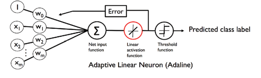
Fig 1. Adaline Linear Activation Function Representation
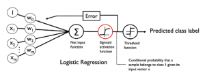
The diagram below represents the activation functions for Logistic Regression. The activation function for Logistic Regression, also called as sigmoid activation function, is the identity function can be represented as the following:
$$\phi(W^TX) = \frac{1}{(1 + e^-Z)}$$

Fig 2: Logistic Sigmoid Activation Function Representation
Difference in Cost Function
For Adaline, the cost function or loss function looks like below:
$$J(w) = \sum\limits_{i} \frac{1}{2} (\phi(z^{(i)}) – y^{(i)})^2$$
For Adaline, the goal is to minimize the above sum of squared error function.
For Logistic regression, the cost function is created based on likelihood function that looks like below:
$$L(w) = P(y \vert x; w) = \prod\limits_{i=1}^n P(y^{(i)} \vert x^{(i)}; w) = \prod\limits_{i=1}^n (\phi(z^{(i)}))^{y^{(i)}} (1 – \phi(z^{(i)}))^{(1-y^{(i)})} $$
For logistic regression, the idea is to maximize the above likelihood function. For ease of calculation and numerical stability the above equation is converted into log-likelihood function which is then maximized. The below represents the log-likelihood function:
$$\log(L(w)) = \sum\limits_{i=1}^n [y^{(i)}\log(\phi(z^{(i)})) + (i – y^{(i)})\log(1 – \phi(z^{(i)}))]$$
The above log-likelihood function could be written in the following manner as the cost function, J(w) that can be minimized using the gradient descent
$$J(w) = \sum\limits_{i=1}^n [-y^{(i)}\log(\phi(z^{(i)})) – (i – y^{(i)})\log(1 – \phi(z^{(i)}))]$$
Note that the superscript represents the ith row. Underscript represents the specific feature in that row.

Check out my latest book titled as First Principles Thinking: Building winning products using first principles thinking.
- Three Approaches to Creating AI Agents: Code Examples - June 27, 2025
- What is Embodied AI? Explained with Examples - May 11, 2025
- Retrieval Augmented Generation (RAG) & LLM: Examples - February 15, 2025
I found it very helpful. However the differences are not too understandable for me