Have you ever wondered why your machine learning model is not performing as expected? Could the “average” behavior of your dataset be misleading your model? How does the “central” or “typical” value of a feature influence the performance of a machine learning model?
In this blog, we will explore the concept of central tendency, its significance in machine learning, and the importance of addressing skewness in your dataset. All of this will be demonstrated with the help of Python code examples using a diabetes dataset.
We will be working with the diabetes dataset which can be found on Kaggle – Diabetes Dataset. The dataset consists for multiple columns such as ‘Glucose’, ‘BloodPressure’, ‘SkinThickness’, ‘Insulin’, ‘BMI’ having 0 as the values. These can be seen as missing value. It would be good to remove these missing values before proceeding ahead with the analysis. The following is the Python code to load the data and remove the missing values.
import pandas as pd

# Load the dataset
df_diabetes = pd.read_csv('/content/diabetes.csv')

# Remove rows where any of the specified columns have a value of 0
columns_to_check = ['Glucose', 'BloodPressure', 'SkinThickness', 'Insulin', 'BMI']
df_diabetes_filtered = df_diabetes[df_diabetes[columns_to_check].apply(lambda row: all(row != 0), axis=1)]

# Show the shape of the original and filtered datasets to indicate how many rows were removed
original_shape = df_diabetes.shape
filtered_shape = df_diabetes_filtered.shape

original_shape, filtered_shape
The original dataset contained 768 rows and 9 columns. After removing rows with zero values in one or more of the specified columns (‘Glucose’, ‘BloodPressure’, ‘SkinThickness’, ‘Insulin’, ‘BMI’), the filtered dataset now contains 392 rows and 9 columns. We will work with df_diabetes_filtered data frame in this blog.
What is Central Tendency & How is it Measured?
Central tendency refers to the measure that identifies the “central” or “typical” value for each feature in a dataset. Three commonly used measures of central tendency are:
- Mean: The mean is perhaps the most commonly used statistic and is calculated by summing up all the values in the dataset and dividing by the number of values. For example, in our diabetes dataset (filtered), the mean insulin level was approximately 156.056 mu U/ml. This value can give us a general idea of the insulin levels in the population, but it’s susceptible to being influenced by outliers. In Python, you can compute the mean using pandas as shown below:
# Calculate the mean of the 'Insulin' feature
mean_insulin = df_diabetes_filtered['Insulin'].mean() - Median: The median is the value that separates the dataset into two equal halves. One half comprises all values that are greater than the median, and the other half comprises values that are less than the median. The median is less affected by outliers and skewed data compared to the mean. Here’s how to calculate it in Python:
# Calculate the median of the 'Insulin' featuremedian_insulin = df_diabetes_filtered['Insulin'].median() - Mode: The mode is the value that appears most frequently in the dataset. A dataset can have zero or more modes. If no number in the list is repeated, then the dataset has no mode. If two numbers appear the same maximum number of times, then the dataset is bimodal. In Python, you can find the mode using pandas:
# Calculate the mode of the 'Insulin' featuremode_insulin = df_diabetes_filtered['Insulin'].mode()[0]
The following Python code can help you get the central tendency for all features in the dataset. The code works for Google Collab if you uploaded the diabetes dataset in the root folder of your jupyter notebook in Google Collab .
# Calculate mean and median for each column
mean_median_stats = df_diabetes_filtered.agg(['mean', 'median']).transpose()

# Calculate mode for each column separately and get the first mode value in case there are multiple modes
mode_stats = df_diabetes_filtered.mode().iloc[0]

# Combine the statistics for display
central_tendency_stats = pd.concat([mean_median_stats, mode_stats.rename('mode')], axis=1)
central_tendency_stats
Here is how the central tendency of all the features would look like:
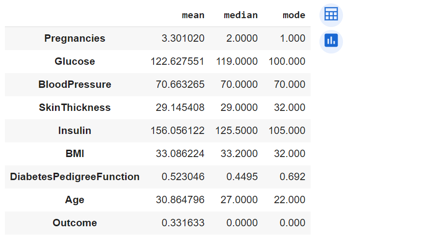
Here are some observations regarding the central tendency measures including mean and median.
- Glucose, BloodPressure, and BMI: The mean and median are quite close, suggesting a more or less normal distribution.
- SkinThickness and Insulin: For Insulin, the mean is higher than the median. This indicates the presence of some skewness in the dataset related to Insulin and needs further investigation.
Let’s review the skewness of ‘Insulin’ feature with visual representation using the following Python code.
import matplotlib.pyplot as plt
import seaborn as sns

# Set up the matplotlib figure
fig, axes = plt.subplots(1, 2, figsize=(14, 5))
fig.suptitle('Distribution and Outliers for Insulin (Filtered Data)')

# Plot histogram for Insulin
sns.histplot(df_diabetes_filtered['Insulin'], kde=True, ax=axes[0])
axes[0].set_title('Histogram of Insulin')

# Plot boxplot for Insulin
sns.boxplot(x=df_diabetes_filtered['Insulin'], ax=axes[1])
axes[1].set_title('Boxplot of Insulin')

plt.tight_layout(rect=[0, 0.03, 1, 0.95])
plt.show()
Here is how the plot would look like:
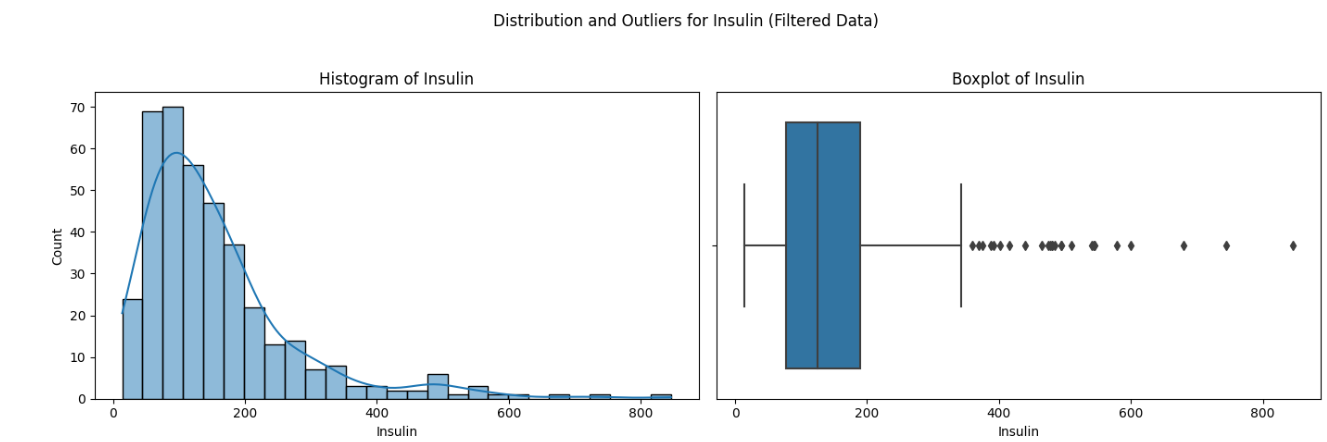
Here are the observations from the above plot:
- Histogram: The data for Insulin in the filtered dataset still shows a right-skewed distribution. The tail towards the higher values is still present, but it’s less pronounced compared to the original dataset.
- Boxplot: The boxplot reveals several outliers on the higher end of the distribution. These outliers are less extreme than those in the original dataset, but they are still present.
The following can be impact on the predictive modeling:
- Skewness: The skewness could affect the performance of models that assume a Gaussian distribution, such as logistic regression models (used for classification).
- Outliers: The presence of outliers can influence the outcome of some models, leading to potentially poor performance.
Why handle Data Skewness & How?
Skewness is a measure of the asymmetry of the probability distribution of a feature. In simpler terms, if the distribution of data is skewed to the left or right, it can impact the machine learning model’s performance. Many machine learning algorithms assume that the data follows a Gaussian distribution. Skewed data can violate this assumption, affecting the model’s performance.
The following can be done as next steps to address the potential challenges posed by skewed data:
- Data transformations like square root, log, or Box-Cox can be applied to address the skewness.
- Outliers can be capped, removed, or transformed to minimize their impact on the model.
The following code demonstrate how we handle data skewness related to Insulin feature.
from scipy.stats import boxcox
import numpy as np
# Prepare data for transformations
insulin_data = df_diabetes_filtered['Insulin']
# Square root transformation
sqrt_transformed = np.sqrt(insulin_data)
# Log transformation
log_transformed = np.log1p(insulin_data) # Using log(1 + x) to handle zero values
# Box-Cox transformation
boxcox_transformed, _ = boxcox(insulin_data)
# Set up the matplotlib figure
fig, axes = plt.subplots(2, 2, figsize=(10, 8))
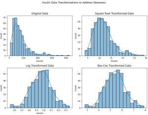
fig.suptitle('Insulin Data Transformations to Address Skewness')
# Plot original data
sns.histplot(insulin_data, kde=True, ax=axes[0, 0])
axes[0, 0].set_title('Original Data')
# Plot square root transformed data
sns.histplot(sqrt_transformed, kde=True, ax=axes[0, 1])
axes[0, 1].set_title('Square Root Transformed Data')
# Plot log transformed data
sns.histplot(log_transformed, kde=True, ax=axes[1, 0])
axes[1, 0].set_title('Log Transformed Data')
# Plot Box-Cox transformed data
sns.histplot(boxcox_transformed, kde=True, ax=axes[1, 1])
axes[1, 1].set_title('Box-Cox Transformed Data')
plt.tight_layout(rect=[0, 0.03, 1, 0.95])
plt.show()
The following is how the plots would look like:
Here are the observations:
- Original Data: The original insulin data is right-skewed, as we observed earlier.
- Square Root Transformed Data: The square root transformation has reduced the skewness to some extent, but a slight right skew is still visible.
- Log Transformed Data: The log transformation has further reduced the skewness, resulting in a distribution that appears closer to a normal distribution.
- Box-Cox Transformed Data: The Box-Cox transformation appears to have done the best job in normalizing the data, resulting in a distribution that is very close to a normal distribution.
The following represents impact on building machine learning model with reduced skewness in the data:
- Reduced Skewness: Transforming skewed data can make it fit better with model assumptions, particularly for models that assume normally distributed data, thus potentially improving model performance.
- Stability: Box-Cox and log transformations often stabilize the variances across levels of an independent variable, which also helps in improving model performance.
Conclusion
Central tendency is not just a statistical concept; it plays a pivotal role in the realm of machine learning and data science. Understanding the mean, median, and mode of your dataset can offer invaluable insights into the ‘average’ behavior of features, thereby influencing the performance of your predictive models. Through our exploration with the diabetes dataset, we saw how these measures can indicate the need for further data preprocessing, such as handling skewness through transformations like Square Root, Log, or Box-Cox. However, as demonstrated, the impact of such transformations can vary depending on the machine learning algorithm being used.

Check out my latest book titled as First Principles Thinking: Building winning products using first principles thinking.
- Three Approaches to Creating AI Agents: Code Examples - June 27, 2025
- What is Embodied AI? Explained with Examples - May 11, 2025
- Retrieval Augmented Generation (RAG) & LLM: Examples - February 15, 2025
I found it very helpful. However the differences are not too understandable for me