
Last updated: 1st May, 2024
The bias-variance trade-off is a fundamental concept in machine learning that presents a challenging dilemma for data scientists. It relates to the problem of simultaneously minimizing two sources of residual error that prevent supervised learning algorithms from generalizing beyond their training data. These two sources of error are related to Bias and Variance. Bias-related errors refer to the error due to overly simplistic machine learning models. Variance-related errors refer to the error due to too much complexity in the models.
In this post, you will learn about the concepts of bias & variance in the machine learning (ML) models. You will learn about the tradeoff between bias and variance which is a fundamental problem in machine learning, and why it is often necessary to experiment with different model types to find the balance between model bias and variance that works best for a given dataset.
What is the Bias-variance tradeoff?
The bias-variance tradeoff is a central problem in supervised machine learning involving two types of error that models can exhibit: bias and variance. Both types of error affect the model’s performance.
It is often impossible to reduce both types of error simultaneously. The challenge is that decreasing one typically increases the other. A highly complex model (low bias) might overfit the training data, capturing noise, and leading to high variance. Conversely, a too-simple model (low variance) might underfit the data, failing to capture underlying patterns, resulting in high bias.
Consequently, careful consideration must be given to the bias-variance tradeoff when designing machine learning models. If the model is too simple, it will suffer from high bias and low variance. If the model is too complex, it will suffer from low bias and high variance. Finding the right balance is essential for creating an effective machine-learning model. The ideal model would have low bias and low variance, but in practice, it is often necessary to trade off one for the other.
Model bias can be lowered using good machine learning algorithms, and feature engineering while making domain-specific adjustments and unbiased training data.
Model variance can be lowered using good machine learning algorithms, a very large set of training data (more than required), and more and less noisy features if possible that are correlated to the target variable.
Model Bias & Variance Intuition
The intuition behind bias and variance can be understood based on the following diagram. One can get a detailed explanation by going through the free online course – Introduction to Machine Learning by Dr. Sebastian Raschka.
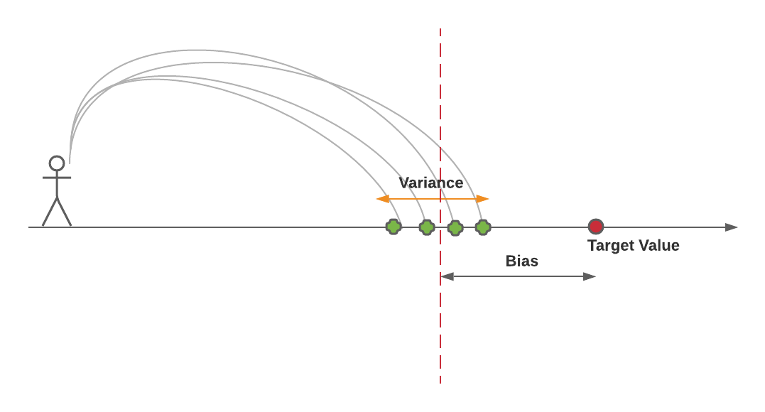
The above diagram represents a person throwing a stone with the goal of hitting the point representing the target value. However, his stones hit the ground at different points much away from the actual / target point. Let’s try and understand bias and variance concepts using the above diagram.
In the above diagram, the bias is represented as the distance between the target value (true value) and the average of points where the stone hit the ground. The dashed line represents the average of predictions made by different models (different points where the stone hit the ground) trained using different training data sets derived from the same population. The lower the distance (and, hence lower bias) between the average (dashed line) and the target value (red circle), the lower the bias, the better is the model. The variance can be represented as the spread of individual points around the average (red dashed line). The lower the spread (and, hence lower variance), the better is the model.
In predictive modeling, bias-variance tradeoff can be understood as a trade-off between simplicity and complexity. On one end, you have the simpler models (high bias), on the other, you have the more complex models (high variance).
Model Loss as a function of Bias & Variance
The total error (or loss) in a predictive model can be broken down into three parts:
$\text{Total Error} = \text{Bias}^2 + \text{Variance} + \text{Irreducible Error}$
- $\text{Bias}^2$: The bias squared term comes from the squared difference between the expected (or average) prediction of the model and the true value. Squaring the bias makes sure that we’re considering how far off the model’s predictions are from the truth, on average, regardless of the direction of the error.
- Variance: This part accounts for the variability in model predictions, reflecting how much the predictions for a given point vary between different versions of the model.
- Irreducible Error: This is the noise term that cannot be reduced by any model.
Balancing Bias and Variance:
- Minimizing Loss: To minimize the total error, one must balance both bias and variance. Too much complexity (low bias, high variance) will fit the noise in the data, whereas too little complexity (high bias, low variance) will fail to capture the underlying pattern.
- Trade-off: Improving bias usually increases variance and vice versa. The key is to find a sweet spot where the increase in one is worth the decrease in the other.
Model Bias & Variance: Ideal Scenarios & Examples
The ideal scenario for model bias and variance in machine learning is achieving a balance where both bias and variance are minimized. This balance is crucial for developing a model that generalizes well to unseen data. Here’s what this ideal scenario entails:
- Low Bias: The model should have enough complexity to capture the underlying patterns and relationships in the training data. This means it can accurately model the important features of the data without oversimplifying them.
- Low Variance: At the same time, the model should not be so complex that it starts fitting the noise in the training data. A model with low variance is not overly sensitive to small fluctuations in the training set and therefore performs consistently across different sets of data.
In machine learning, if the ideal balance of low bias and low variance is unattainable, the second best scenario typically involves prioritizing one over the other based on the specific requirements and constraints of the problem at hand. This decision is often influenced by the nature of the data, the application domain, and the cost of errors. The two common second-best scenarios are:
- Prioritizing Low Bias (Accepting Higher Variance):
- When Applicable: This approach is suitable when the cost of missing underlying patterns (underfitting) is higher than the cost of overfitting. It’s often chosen in complex problems where capturing the nuances in the data is crucial.
- Example: In medical diagnostics or financial forecasting, missing out on critical patterns could have serious consequences, so a model with slightly higher variance but lower bias might be preferable.
- Prioritizing Low Variance (Accepting Higher Bias):
- When Applicable: This scenario is chosen when it’s more important for the model to be consistent across various datasets, even if it means not capturing all patterns perfectly. It’s common in applications where overfitting to noise or outliers can lead to significant problems.
- Example: In spam detection systems, it might be preferable to have a model that consistently identifies most spam across different datasets, even if it means some spam emails are missed (high bias), rather than a model that overfits to the training data and performs inconsistently in real-world applications.
What is bias in machine learning models?
The bias in machine learning is a concept that describes how far a model’s predictions are from the actual values. It arises when a model is too simple and makes assumptions that don’t capture the complexity of the underlying data, resulting in underfitting. Underfitting occurs when a model is not able to model the data well enough, meaning it doesn’t perform well on the training data, and as a result, also performs poorly on new, unseen data.
High model bias may mean that the model is making wrong predictions because it might have missed certain important features. In other words, the model has been under-fitted. Low model bias would mean that the model may have considered important features apart from other less important ones while being trained. The following picture demonstrates the model bias for linear and polynomial regression model.
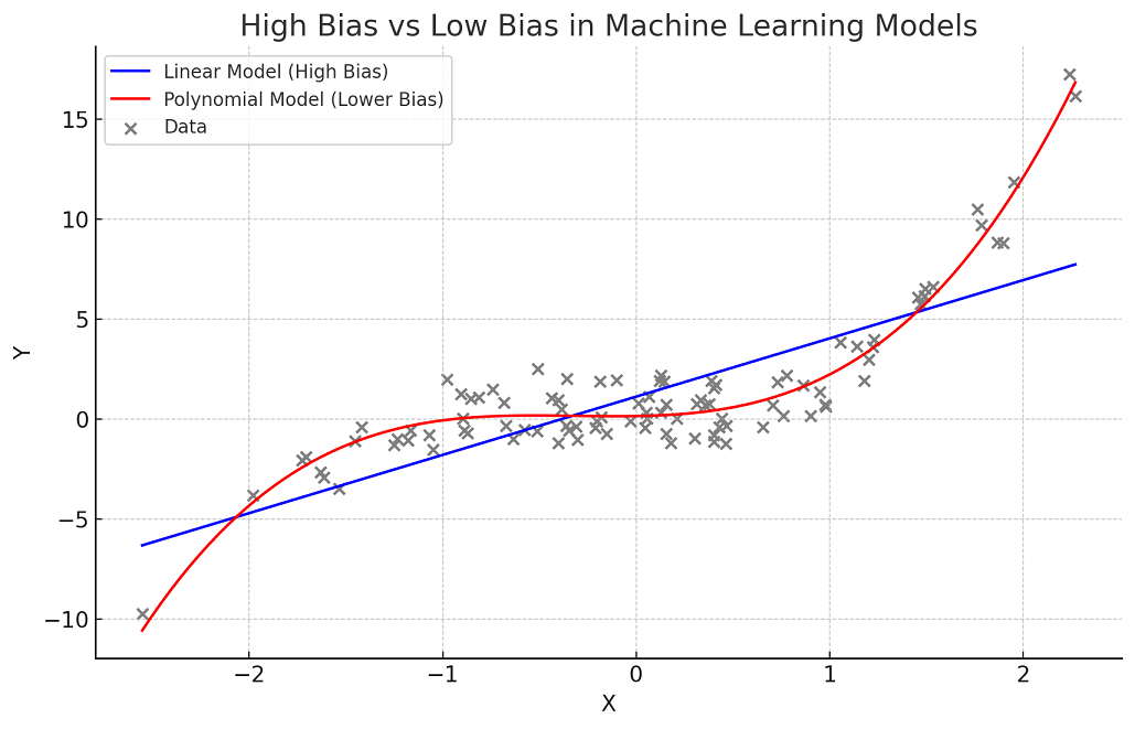
Here’s the plot demonstrating high bias and low bias scenarios in machine learning models:
- Linear Regression Model (Blue Line) having Higher Bias: This line represents a linear regression model’s prediction. It is a simple model and assumes a linear relationship between X and Y. However, the actual relationship is non-linear, so the linear model, with its high bias, fails to capture this complexity, leading to underfitting. This is evident as the blue line does not follow the curved pattern of the data points.
- Polynomial Regression Model (Red Line) having Lower Bias: This line shows the prediction of a polynomial regression model, which has lower bias compared to the linear model. It is able to capture the non-linear relationship more effectively, fitting the data much better than the linear model.
Model Bias Formula
Mathematically, the bias of the model can be represented using the following equation:
$\Large Bias = E[\hat{\theta}] – \theta$
In the above equation, the $E[\hat{\theta}]$ represents the expected value of the prediction which is an average of predictions made by different estimators, and, $\theta$ represents the true value.
What is variance in machine learning models?
The concept of variance in machine learning models relates to how much the predictions of a model vary for a given data point when the model is trained on different subsets of the same dataset. Since the training data are used to fit the machine learning models using a set of hyperparameters, different training data sets with different sets of hyperparameters will result in different models.
High variance indicates that the model’s predictions are highly sensitive to the specific data it was trained on, leading to overfitting. The ideal model will tend to have low variance. In other words, the ideal model will be the one whose predictions would not vary too much between training sets. However, if a model has high variance then small changes in the training data can result in large changes in the model prediction performance.
Model Variance Formula
Mathematically, variance can be represented as the following:
$\Large Var = E[{\hat{\theta}}^2] – {E[\hat{\theta}]}^2$
Above equation can also be expressed as the following:
$\Large Var = E[(E[\hat\theta] – \hat\theta)^2]$

Check out my latest book titled as First Principles Thinking: Building winning products using first principles thinking.
- Mathematics Topics for Machine Learning Beginners - July 6, 2025
- Questions to Ask When Thinking Like a Product Leader - July 3, 2025
- Three Approaches to Creating AI Agents: Code Examples - June 27, 2025
I found it very helpful. However the differences are not too understandable for me