In this post, you will learn about the concepts of Bernoulli Distribution along with real-world examples and Python code samples. As a data scientist, it is very important to understand statistical concepts around various different probability distributions to understand the data distribution in a better manner. In this post, the following topics will get covered:
- Introduction to Bernoulli distribution
- Bernoulli distribution real-world examples
- Bernoulli distribution python code examples
Introduction to Bernoulli Distribution
Bernoulli distribution is a discrete probability distribution representing the discrete probabilities of a random variable which can take only one of the two possible values such as 1 or 0, yes or no, true or false etc. The probability of random variable taking value as 1 is p and value as 0 is (1-p). In Bernoulli distribution, the number of trials is only 1. The one trial representing Bernoulli distribution is also termed as Bernoulli trial. Bernoulli distribution is also considered as the special case of binomial distribution with n = 1 where n represents number of trials.
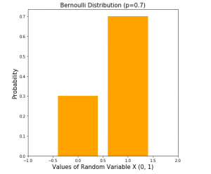
Here is a sample diagram that represents a Bernoulli Distribution with probability value, p = 0.7 for k = 1

Bernoulli trial is a random experiment whose outcome can only be one of the possible values such as success or failure. The outcome of Bernoulli trial is called as Bernoulli random variable. The outcome of interest is termed as success. Thus, for a Bernoulli trial of a coin toss, the outcome of interest is head. Thus, success is associated with head appearing after coin is tossed. The probability of getting success is p and failure is 1 – p. For a coin toss, the probability of getting head (or success) is 0.5. Thus, the probability of getting tail is 1 – 0.5 = 0.5.
As the Bernoulli distribution is a discrete probability distribution, the probabilities of different value of random variable can be determined using the following probability mass function (PMF):
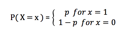
The expected value of the Bernoulli random variable is p which is also called as the parameter of the Bernoulli distribution. The variance of the values of Bernoulli random variable is p(1-p).
Bernoulli Distribution Real-world Examples
Here are some real-world examples of Bernoulli distribution. Remember that all we need to look for is random experiment which could have only two possible outcomes as success or failure. The outcome of interest is denoted as success. It is important to define what is your experiment and what means success if the experiment is done.
- Coin toss with only two possible outcomes – head or tail. Success = 1 if coin shows up head. X = {head, tail}
- Rolling a die resulted in 6 or not. Success = 1 for die = 6
- Whether a person voted for a particular political party or abstained from voting. Success = 1 if voted for a political party
- Whether a student got more than 80 marks or not. Success = 1 if marks > 80
- From a bag consisting of red, green and black ball, when a ball is taken out, whether the ball taken out has red color or not. Success = 1 if the color of ball taken out is red.
- Whether the outcome of interview is recommendation for next round of interview or not. Success = 1 if the outcome of interview is recommendation to next round of interview.
Bernoulli Distribution Python Code Examples
Here is the Python code representing the Bernoulli distribution and usage of probability mass function to create the bar plot. Pay attention to some of the following in the code below:
- Python Scipy Bernoulli class is used to calculate probability mass function values
- Instance of Bernoulli distribution with parameter p = 0.7
- Outcome of experiment can take value as 0, 1. The values of Bernoulli random variable can take 0 or 1.
- The usage of pmf function to determine the probability of different values of random variable
import matplotlib.pyplot as plt
from scipy.stats import bernoulli
#
# Instance of Bernoulli distribution with parameter p = 0.7
#
bd = bernoulli(0.7)
#
# Outcome of experiment can take value as 0, 1
#
X = [0, 1]
#
# Create a bar plot; Note the usage of "pmf" function
# to determine the probability of different values of
# random variable
#
plt.figure(figsize=(7,7))
plt.xlim(-1, 2)
plt.bar(X, bd.pmf(X), color='orange')
plt.title('Bernoulli Distribution (p=0.7)', fontsize='15')
plt.xlabel('Values of Random Variable X (0, 1)', fontsize='15')
plt.ylabel('Probability', fontsize='15')
plt.show()
The above code when executed results in the plot shown in fig 1.
Conclusions
In this post, you learned about some of the following in relation to Bernoulli Distribution:
- Bernoulli distribution is discrete probability distribution representing the probabilities of getting different / discrete values of the random variable. The random variable could take only two possible values such as success or failure. The random variable is also termed as Bernoulli random variable.
- Bernoulli distribution represents the probabilities of two possible outcomes of a single random experiment
- The single random experiment is termed as Bernoulli trial.
- The mean or expected value of the Bernoulli distribution is p and variance is p(1-p)

Check out my latest book titled as First Principles Thinking: Building winning products using first principles thinking.
- Questions to Ask When Thinking Like a Product Leader - July 3, 2025
- Three Approaches to Creating AI Agents: Code Examples - June 27, 2025
- What is Embodied AI? Explained with Examples - May 11, 2025
I found it very helpful. However the differences are not too understandable for me