In this post, you will learn about Beta probability distribution with the help of Python examples. As a data scientist, it is very important to understand beta distribution as it is used very commonly as prior in Bayesian modeling. In this post, the following topics get covered:
- Beta distribution intuition and examples
- Introduction to beta distribution
- Beta distribution python examples
Beta Distribution Intuition & Examples
Beta distribution is widely used to model the prior beliefs or probability distribution in real world applications. Here is a great article on understanding beta distribution with an example of baseball game. You may want to pay attention to the fact that even if the baseball player got strikeout in first couple of matches, one still may chose to believe based on his prior belief (prior distribution) that he would end up achieving his batting average. However, as the match proceed, the prior may change based on his performance in subsequent matches. This would mean altering the parameters value of [latex]\alpha[/latex] and [latex]\beta[/latex].
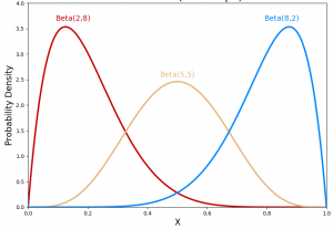
If there exists a prior distribution about any event having outcome within an interval (a < X < b or 0 < X < 1), based on the upcoming event outcomes, the prior may change. The diagram below represents the hypothetical scenario representing the change in prior probability distribution which happens due to change in the value of shape parameters value of [latex]\alpha[/latex] and [latex]\beta[/latex].

Once the shape parameters, [latex]\alpha[/latex] and [latex]\beta[/latex] get determined, one could use the probability density function to determine the probability of event having with value of random variable falling within a given interval. Let’s understand this with an example. Let’s say you create a beta distribution to model the percentage of votes a particular politician would get in an upcoming interval. Once the shape parameters’ values of [latex]\alpha[/latex] and [latex]\beta[/latex] are known, one could find out the value that the politician will get votes falling between percentage ranges.
Introduction to Beta Distribution
Beta distribution is continuous probability distribution representing probabilities of the random variable which can have only finite set of values. This is unlike other probability distributions where the random variable’s value can take infinity as values, at least in one direction.
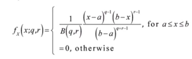
Beta distribution have two shape parameters namely [latex]\alpha[/latex] and [latex]\beta[/latex]. The random variable in beta distribution can have values between finite set of values such as a and b or 0 and 1. When the random variable has value between a and b and parameters [latex]\alpha[/latex] and [latex]\beta[/latex], the beta distribution is termed as general beta distribution. Given the fact that there are four parameters to be determined, it is also termed as four parameters beta distribution. Here is the probability distribution function for 4-parameters beta distribution. Note the parameters a, b, q as [latex]\alpha[/latex] and r as [latex]\beta[/latex]. B(q, r) is beta function. Note that the shape parameters are always positive.
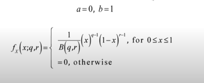
When the random variable can have values between 0 and 1 and parameters [latex]\alpha[/latex] and [latex]\beta[/latex], the beta distribution is termed as standard beta distribution. Given the fact that there are two parameters to be determined, it is also termed as two parameters beta distribution. A four-parameters or general beta distribution can be transformed into two-parameters or standard beta distribution. Recall normal distribution and standard normal distribution (mean as 0 and standard deviation as 1). Here is the probability distribution function for standard beta distribution or 2-parameters beta distribution. Pay attention to a and b taking value as 0 and 1 respectively. The shape parameters are q and r ([latex]\alpha[/latex] and [latex]\beta[/latex])
Here is the probability distribution diagram for standard beta distribution (0 < X < 1) representing different shapes. Note that for different values of the parameters [latex]\alpha[/latex] and [latex]\beta[/latex], the shape of the beta distribution will change.
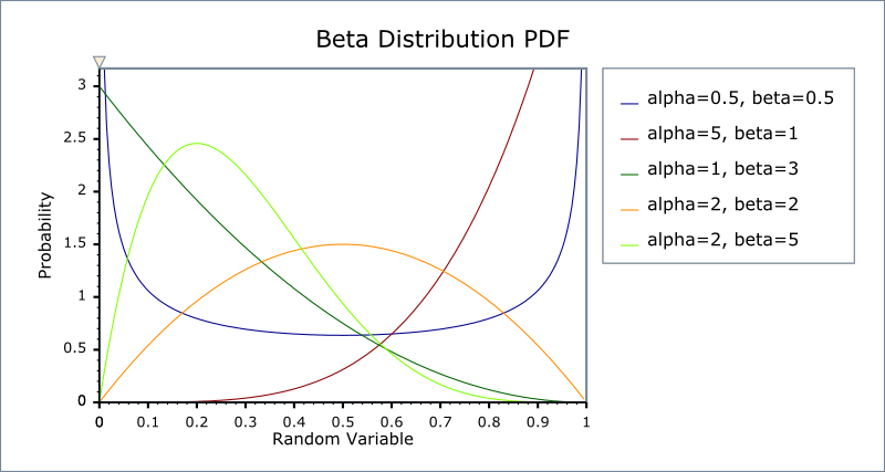
The very fact that the beta distribution can have different shapes based on different values of parameters make this distribution very useful. Also, for random variable having values between 0 and 1, beta distribution can be used to model probabilities whose values lie between 0 and 1. Thus, for modeling probabilities, both the X axis and Y axis represent probabilities. For that matter, standard beta distribution can also be termed as probability distribution of probabilities.
Given the fact that standard beta distribution is used to model probability distribution of probabilities, it is most commonly used as prior in Bayesian modeling.
The mean of beta distribution is [latex]\frac{\aplha}{\alpha + \beta}[/latex].
As beta distribution is used as prior distribution, beta distribution can act as conjugate prior to the likelihood probability distribution function. Thus, if the likelihood probability function is binomial distribution, in that case, beta distribution will be called as conjugate prior of binomial distribution.
Beta Distribution Python Examples
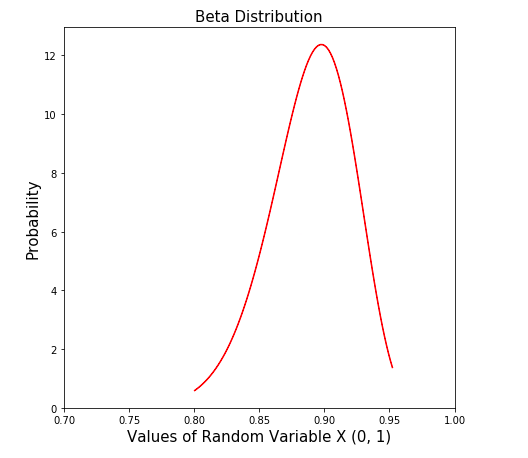
Here is the Python code which can be used to create beta distribution.
import numpy as np
import matplotlib.pyplot as plt
from scipy.stats import beta
#
# Set the shape paremeters
#
a, b = 80, 10
#
# Generate the value between
#
x = np.linspace(beta.ppf(0.01, a, b),beta.ppf(0.99, a, b), 100)
#
# Plot the beta distribution
#
plt.figure(figsize=(7,7))
plt.xlim(0.7, 1)
plt.plot(x, beta.pdf(x, a, b), 'r-')
plt.title('Beta Distribution', fontsize='15')
plt.xlabel('Values of Random Variable X (0, 1)', fontsize='15')
plt.ylabel('Probability', fontsize='15')
plt.show()
Here is how the plot would look like for above code:
References
Conclusions
Here is the summary of what you learned in this post in relation to beta distribution:
- Beta distribution can be used to model probability distribution of probabilities
- Beta distribution is more often used in the Bayesian modeling
- When four parameters such as inner and outer bound of interval and [latex]\alpha[/latex] and [latex]\beta[/latex] are unknown, the beta distribution is known as general beta distribution or four-parameters beta distribution.
- When two parameters such as [latex]\alpha[/latex] and [latex]\beta[/latex] are unknown and interval varies between 0 and 1, the beta distribution is known as standard beta distribution or two-parameters beta distribution.

Check out my latest book titled as First Principles Thinking: Building winning products using first principles thinking.
- Mathematics Topics for Machine Learning Beginners - July 6, 2025
- Questions to Ask When Thinking Like a Product Leader - July 3, 2025
- Three Approaches to Creating AI Agents: Code Examples - June 27, 2025
Just began learning python: trying to understand how to solve/code: finding the MLE of a histogram using the scipy.stats.beta class. The true parameters are a=4, b=2 using the raw data?