Last updated: 12th May, 2024
In the world of generative AI models, autoencoders (AE) and variational autoencoders (VAEs) have emerged as powerful unsupervised learning techniques for data representation, compression, and generation. While they share some similarities, these algorithms have unique properties and applications that distinguish them. This blog post aims to help machine learning / deep learning enthusiasts understand these two methods, their key differences, and how they can be utilized in various data-driven tasks. We will learn about autoencoders and VAEs, understanding their core components, working mechanisms, and common use cases. We will also try and understand their differences in terms of architecture, objectives, and outcomes.
What are Autoencoders?
An autoencoder is a type of generative model that is used for unsupervised learning of high dimensional input data representations into lower dimensions embedding vector with the goal of recreating or reconstructing the input data. In other words, the primary goal of the Autoencoder is to learn a compressed, latent/hidden representation of input data and then reconstruct the input data from this lower-dimensional representation with minimal loss of information.
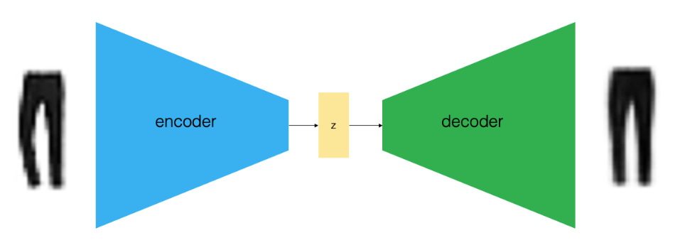
Based on the above, you may note that an autoencoder architecture consists of three main components.
- Encoder: The encoder represents a deep neural network comprising of one or more stacked convolutional layers which are used to compress the high dimensional dataset (trouser image) to a low dimensional embedding vector. Here is what the one form of encoder network architecture might look like. Note a bunch of 2-dimensional convolutional layers are stacked and used along with parameters trained for each of these layers. The embedding space is the last two-dimensional “Dense” layer.

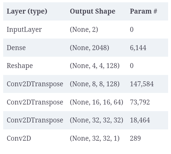
- Decoder: The Decoder represents the deep neural network comprising one or more stacked transposed convolutional layers. This network decompresses a given embedding vector back to the same or new image. One or more transposed convolutional layers with appropriate kernels are trained. Here is one form of decoder network architecture. Note multiple transposed convolutional layers and the image is last Dense layer having 32 x 32 pixel with grayscale channel.
- Embedding space or latent space denoted using z: The embedding space is a compression of the original image into a lower-dimensional space. It is used to create new images based on sampling different points and passing the points through the decoder network. The decoder has learned appropriate transposed convolutional filters to create new images from points in the embedding space. Thus, when new points are sampled and passed through the decoder network, new viable images get created.
In order to train the encoder decoder network (autoencoder), a model gets defined which represents the flow of an image from an encoder to a decoder network. The Keras code such as the following represents the idea.
#
# Autoencoder model definition
#
autoencoder = Model(encoder_input, decoder(encoder_output))
#
# Compile the autoencoder model
#
autoencoder.compile(optimizer="adam", loss="binary_crossentropy")
#
# Fit the model
#
autoencoder.fit(x_train, x_train, epochs=5, batch_size=100, shuffle=True, validation_data=(x_test, x_test))
Once the model gets trained, one can reconstruct the image using the following code:
example_images = x_test[:5000]
predictions = autoencoder.predict(example_images)
The autoencoder results in latent space such as the following where each point is a representation of encoding of an image which when decoded results in same or new images.
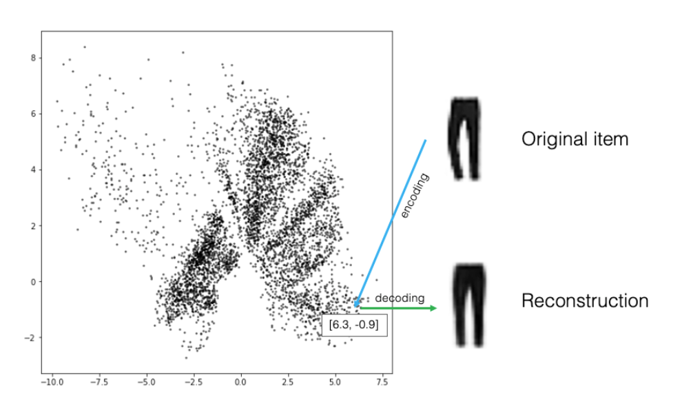
However, there are a few issues with the above due to which variational autoencoders got invented. Let’s look at these issues:
- The distribution of points is non-symmetrical. Thus, there is a challenge in how do we go about selecting a point to create the images we desire.
- Some types of images get encoded over a very small area and others over a larger area. Thus, if a point is sampled randomly in the embedding space, it is more likely to create an image which looks like the type of images encoded over larger area.
- There are areas called holes with no points between the images of different types. Thus, if a point is randomly picked up from this space, it is not certain whether the desired images will be created. Autoencoder has no way to ensure that the points in the latent space are continuous.
As the number of dimensions increases, the above issues become more amplified. This is where variational autoencoders come into the picture. They help address the issues not dealt by the vanilla autoencoders.
What are Variational Autoencoders (VAE)?
Variational autoencoders are a class of generative and probabilistic models that extend the concept of autoencoders by introducing probabilistic encoding and decoding. The following are some of the distinct characteristics that make it different from the traditional autoencoders:
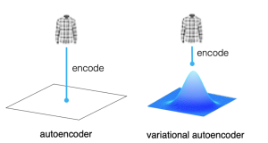
- Mapping input image to a distribution rather than a point in the latent space: As learned in the previous section, in an autoencoder, the input image is encoded into a single point in the latent space through the encoder network, which then decodes the point to reconstruct the original input image. On the other hand, a variational autoencoder (VAE) maps the input image to a distribution in the latent space, rather than a single point. In other words, the encoder maps each input to a mean vector and a variance vector. Specifically, it maps the input to a multivariate normal distribution around a point in the latent space, which captures the variability of the data. This means that instead of learning a single encoding for each input, the VAE learns a distribution of encodings that can represent the input image with some degree of uncertainty. This allows the VAE to learn a richer representation of the input data that can be used for various generative tasks. The picture below represents the concept:

To illustrate this, let’s consider an example of image generation. Suppose we want to generate new images of a specific class, say, a shirt. We can train a VAE on a dataset of shirt images, and sample random points from the learned distribution in the latent space. These points can then be decoded by the VAE’s decoder network to generate new shirt images that share similar characteristics with the original dataset. The use of a multivariate normal distribution allows the VAE to generate diverse images that still belong to the same class. On the other hand, when we use the autoencoder, the point next to a given point may end up creating an image which is not of similar type.
Here is how the VAEs do the task:
1. The encoder takes an input data point and maps it to a probability distribution in a lower-dimensional latent space. The input data is encoded into mean and variance vectors representing the parameters of a multivariate Gaussian distribution in the latent space.
2. Data is then represented in the latent space that captures the underlying structure of the data.
3. The next step is the decoding phase, where the model takes a sample from the latent space and maps it back to the original data space.
4. The training process of the VAE entails a minimization of a loss function (reconstruction loss + KL divergence term) which is discussed in the next point. - Different loss function for variational autoencoder: The other difference between autoencoder and variational autoencoder is the usage of the loss function. In an autoencoder, the loss function only consists of the reconstruction loss between the input and its corresponding output generated by the encoder-decoder pair. The objective of the autoencoder is to minimize this loss, which means that it tries to reconstruct the input image as accurately as possible. On the other hand, the loss function for a VAE includes two components: the reconstruction loss and the Kullback-Leibler (KL) divergence term. The reconstruction loss measures the difference between the input image and its reconstructed version, similar to the autoencoder. However, the KL divergence term measures how different the learned distribution of the latent variables is from the prior distribution, which is usually assumed to be a standard normal distribution. This regularization term helps the VAE to avoid overfitting and to learn a more robust latent space.
Recall that Kullback-Leibler (KL) divergence term is a measure of how much one probability distribution differs from another. In the context of variational autoencoders (VAEs), the KL divergence term is used as a regularization term in the loss function. The purpose of this term is to encourage the learned latent variables to follow a prior distribution, which is usually assumed to be a standard normal distribution. This prior distribution can help the VAE to generate diverse and realistic samples by forcing the learned distribution to be more structured.
More specifically, in a VAE, the encoder network maps the input data to a distribution over the latent variables, with mean and variance parameters (z_mean, z_log_var with z representing embedding space). The decoder network then maps the sampled latent variables back to the input space. The objective of the VAE is to minimize the reconstruction loss, which measures the difference between the input and its corresponding output generated by the encoder-decoder pair, and the KL divergence term, which measures the difference between the learned distribution and the prior distribution.
To illustrate the concept around reconstruction loss and KL divergence term, let’s consider an example of image generation using a VAE. Suppose we want to generate new images of a specific class, say, birds. We can train a VAE on a dataset of bird images and sample random points from the learned distribution in the latent space. The KL divergence term ensures that the sampled points are within the learned distribution and not too far from the prior distribution, which can help the VAE generate more diverse and realistic images.
Conclusion
In conclusion, the difference between Autoencoder and Variational Autoencoder is significant. While in the case of autoencoders, the encoder network maps input data to a fixed point, in case of variational autoencoders, the encoder network maps input data to a distribution (multivariate normal distribution). Additionally, the loss function of the variational autoencoder includes an additional KL divergence term in addition to the reconstruction loss. The use of the variational Autoencoder has revolutionized the field of generative modeling by allowing for the generation of new data points by sampling from the learned latent space. The addition of the KL divergence term ensures that the learned distribution is close to a prior distribution, which is essential for generating diverse and meaningful samples.
If you are interested in learning more about Autoencoders and Variational Autoencoders, do not hesitate to reach out for further clarification. There are numerous resources available, and understanding these models’ differences can help you make informed decisions about which model to use for specific applications.

Check out my latest book titled as First Principles Thinking: Building winning products using first principles thinking.
- Questions to Ask When Thinking Like a Product Leader - July 3, 2025
- Three Approaches to Creating AI Agents: Code Examples - June 27, 2025
- What is Embodied AI? Explained with Examples - May 11, 2025
I found it very helpful. However the differences are not too understandable for me